Download
1 / 18
180 likes | 374 Views
Measures of Spread (or Variability or Dispersion). Dispersion. Dispersion refers to how much the data are spread out. Analogy: In terms of physical fitness, a person which can do the “splits” is more agile than one who can not. The agile one can spread out more!

E N D
Measures of Spread (or Variability or Dispersion)
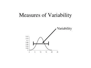
Dispersion Dispersion refers to how much the data are spread out. Analogy: In terms of physical fitness, a person which can do the “splits” is more agile than one who can not. The agile one can spread out more! Data sets that are more disperse are spread out more. Other names for dispersion are variability, variation or spread. So, when we look at a variable we can look at the variation. This is the amount of scattering of the values away from the central value.
The Range The range is a measure of dispersion and can be found by largest value on a variable minus the smallest value. For example the range of the data set 1, 3, 5 is 5 minus 1 = 4. The range as a measure of variability has a problem in that the lowest and the highest numbers could be far away from the rest of the data. This would suggest more variability than perhaps there really is in the data. Next I want to look at the interquartile range as a measure of spread, but I first tell you about percentiles.
Percentiles A percentile is a measure of relative standing, meaning we get information about the position of a value relative to the rest of the data set.
An example: last 10 golf scores for 18 holes, sorted: 82, 83, 84, 85, 85, 88, 90, 90, 93, 95 1 2 3 4 5 6 7 8 9 10 Here I have an example where I wrote down the last 10 golf scores I had. Note that I have sorted the scores from low to high score (although that is not the order I shot them – but for what I want to do next I need to have the data sorted from low to high – ascending order). Below each score I put the “location” of the score in the ascending order.
Here is an approximation method to get percentiles. Let p = the percentile of interest, n = the number of data points or observations, then Lp = (n + 1)(p/100)n is a location index number (a fancy name for a handy little device) we will use to find pth percentile. Now, if n = 10 and if we want the 25th percentile the location index is Lp = (10 + 1)(25/100) = 11(.25) = 2.75. In my example data points have locations with whole numbers. The location index of 2.75 is between 2 and 3. The 25th percentile value will be 75% of the way between the 2nd and 3rd number.
The 2nd number is 83 and the third number is 84. To get the 25th percentile number take the lower number, 83 and add .75 of the difference between the 2nd and 3rd numbers: 83 + .75(84 – 83) = 83.75. Note if the index is a whole number the value in that location is the percentile of interest. The 50th percentile here is found by: Lp = (10 + 1)(50/100) = 5.5 or half the way between the 5th and 6th numbers. So, 85 + .5(88 – 85) = 86.5 is the 50th percentile.
Quartiles Quartiles are just special percentiles. The 25th percentile is the 1st quartile, the 50th percentile is the 2nd quartile (and also called median) and the 75th percentile is the 3rd quartile. What is most important here, I think, is that you understand the meaning of a percentile and the special percentiles called quartiles. So the meaning of the ith percentile is that in the data set that has been arranged from low to high value the ith percentile is the value such that i percent of the cases have this value or less! In my golf score example, the 25th percentile of 83.75 means that out of my last 10 scores 25 percent or fewer of the scores were less than 83.75.
special percentiles • The 25th and 75th percentiles are called the 1st and 3rd quartiles(Q1 and Q3), respectively. They are just the medians of the lower and upper halves of the arranged values. The following is a visual to see the percentiles. lowest next next highest 25% 25% 25% 25% of observations number line where we measure values of the variable first quartile is a value median is a value third quartile is a value
Interquartile range • Variation can be indicated by the interquartile range, IQR = Q3 - Q1. The smaller the IQR, the closer Q3 and Q1 are in the graph and thus the lower the spread! • Hey, please check out the box plot, or what is sometimes called the box and whiskers plot in the text. I know you will! This plot is based on the 5 number summary.
standard deviation • The standard deviation is, perhaps, the most common measure of spread reported. • It is related to the concept called the variance in that the standard deviation is the square root of the variance. • Example: What is the square root of 9? 3 - no biggie! • The standard deviation is used so much because it is useful in visually understanding the normal distribution. We will see this later.
On the next screen I have pointed out an example and I will use the following notation: xi xi - x (xi - x)2 xi is just the ith data value, x is the mean of the data, and (xi - x)2 is the mean subtracted from a data value and then squared. As an example, say the a data value is 6 and the mean of the data is 7. Then we would have (6 – 7 )2 = (-1)2 = 1 A deviation is a data value minus the mean. If you think about it, a deviation is just a distance on the number line. 6 – 7 = -1 means 6 is one unit away from the mean, and the minus sign means on the low side of the mean. (6 – 7 )2 is just a deviation squared, or a squared deviation.
standard deviation • Let’s do some simple examples I have made up to see what is going on. • Note below we have three observations, the values of x are 6, 7, 8 and the average of the three numbers is 7. obs xi xi - x (xi - x)2 1 6 6 - 7 1 2 7 7 - 7 0 3 8 8 - 7 1 Σ(xi - x)2 = 2 The sum of the squared deviations. So the variance is 2/2 = 1 (I show how in a few slides), where the denominator is n-1 (the number of numbers minus 1). The standard deviation is thus sqrt(1) = 1.
standard deviation • Here is another simple example. Note below we have three observations, the values of x are 5, 7, 9 and the average of the three numbers is 7. • The previous example had numbers 6, 7, 8, numbers not spread out as much on the number line. We will see obs xi xi - x (xi - x)2 the numbers 5, 7, 9 have 1 5 5 - 7 4 a larger standard 2 7 7 - 7 0 deviation. 3 9 9 - 7 4 Σ(xi - x)2 = 8 So the variance is 8/2 = 4. The standard deviation is thus sqrt(4) = 2.
standard deviation notes about simple examples • Both examples have sample mean of 7. • The first example has values closer to 7 and it had the smaller calculated standard deviation. • So, the closer the values of the variable are to the mean, the smaller is the standard deviation - the smaller the spread!
Variances and Standard Deviations Remember we want to think about variability here. Variance and standard deviation are related in that the standard deviation is the square root of the variance. How do we interpret these concepts. At this point I think we need to just put them in the context of two data sets. The data set with a larger variance (or standard deviation) will be the one that is more spread out – has more variability. Remember: Data set a = 6, 7, 8. Data set b = 5, 7, 9 By the variance measure data set b is more spread out. By the way, in the variance and standard deviation calculations the sum of the squares of the deviations of the data values from the mean is often just called the sum of squares – SS.
Population and Sample The population variance and standard deviations are based on adding the squared deviations. In fact, the variance is just the average of the squared deviations. In symbols, the population variance is σ2 = Σ(xi – μ)2/N The sample variance is similar, s2 = Σ(xi – x)2/(n-1). Remember N = population size, n = sample size. Note in the sample variance there is division by n-1. Why? Later when we do inference procedures dividing by n-1 makes the resulting sample variance a better way to estimate the population variance.
The Coefficient of Variation By definition, the coefficient of variation is (standard deviation/mean)100. Let’s think about an example of the monthly salary of some recent graduates. Say the mean is $2940 and the standard deviation is 165.65. Then the coefficient of variation is (165.65/2940)100 = 5.6 Thus, the sample standard deviation is only 5.6% of the sample mean. Why even have this crazy measure? This is a useful measure when comparing the variability of variables that have different standard deviations and different means.