About data assimilation
460 likes | 607 Views
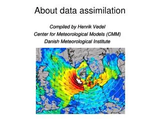
About data assimilation. Compiled by Henrik Vedel Center for Meteorological Models (CMM) Danish Meteorological Institute. NWP is an” initial value problem”.

About data assimilation
E N D
Presentation Transcript
About data assimilation Compiled by Henrik Vedel Center for Meteorological Models (CMM) Danish Meteorological Institute
NWP is an” initial value problem”. Weneed a NWP model field to start an NWP model simulation from. This field is to represent the currentstate of the atmosphere as precisely as possible, given the variables of the model and its resolution. To find determinethisfieldweneed observations.
Atmospheric motion vectors (based on geostationary satellites)
MENU Ingredients of DMIs numerical weather prediction system Computer generated forecasts (fx byvejr) Boundary values from external model Observations Data assimilation system provide ”Analysis” (=initial conditions) Numerical weather model Forecasts by forecasters (fx landsudsigt og regionaludsigter) Old model state Combined and done on a very powerfull computer
Example: HIRLAM S03/SKA details • HIRLAM = High Resolution Limited Area Model • Boundary conditions = ECMWF global model • Horizontal grid resolution = 0.03° (approx 3 km) • Vertical layers = 65 • Grid points = 978 * 818 * 65 • Approximately 8 variables • Forecast length=54h, time step=90s • Runs on 50 nodes (700 cores) using MPI parallelization; asynchronous I/O on 8 cores
Data assimilation • The initial state is not based solely on observations, because: • The problem is vastly under determined in terms of available observations. • The model has skill that should not be thrown away. It is far better than interpolation between observations. • Many newer type observation types do not correspond directly to model variables (wind, temperature, humidity, surface pressure, specific humidity, etc (or similar)), but rather a combination thereof. They can only be properly assimilated with the help of the model field.
Data assimilation • The process of determining the initial state is called data assimilation • The result, the new initial state, is called the analysis.
In a data assimilation system based on variationalanalysis (VAR), the observations and NWP model firstguessfieldarecombined in a statistically optimal way. • Provided the assumptionsabout the size of errors and their distributions arecorrect, the result is the maximumlikelihoodestimate of the atmosphericstate. • It is muchmuchbetterthan the estimateprovided by any single observing system. • A mainbenefit of the VAR formulation, is that observations do not need to correspond to model variables to beassimilated. Any observation type whichcanbeestimated from the model data canbeassimilated. Alsovery ”abstract” observations, such as satelliteradiances, GNSS radio occultations, and GNSS zenithdelays, whichdepend on many model variables from extended parts of the model. • The use of variational data assimilation has lead to a hugeincrease in the types of observations used, and areresponsible for a significant part of the improved NWP skill in the last decades.
Impact of different observations on different scales in Meteo France Arome Slide from Pierre Brousseau, Météo France
Handling of observation errors • On the NWP side wehopethat the observation data providers have done basic checks of the observations. In practice it varies, and we do not rely on it. • There is a somewhatrudimentary check on data in the reading in phase – checkingwhether the expected information is found, sometimes check againstclimatology, etc. • The mainqualityestimation is done in the firstguess check. Here the observation is compared to the expectionvaluebased on the firstguess model state. If the deviation is large, i.e. 5 time the assumed observation error, the observation is consideredlikelyerrorneous, and is not included as active in the data assimilation. If the observation is close to this limit, it is given a lowerweight. • The setup is used for a presetnumber of iteration steps in the minimalisation of J. Then the procedure of check against deviation from the NWP model estimate is done again, possibly resulting in a change of the active stations and/or theirweightsdepending on the setup. • This works fine in general. But thereareexampleswhereone, or a few, correct observations thatcould have corrected a faulthyforecast of servere weatherwasthrown out by the firstguess check.
Data assimilation time window, cut-off time, and NWP cyclingfrequency • The ”data assimilation time window ” is the theperiod from withinwhich observations areselected for data assimilation in a given model setup. • In 3DVar onlyone observation per site and type within the time window is chosen for assimilation , the oneclosest to the valid time of the analysis = valid time of firstguess. Henrce for highfrequency observations manyare not used. • In 4DVar the full DA time window is brokeninto sub windows, eachtypically 1 h in length. Within the sub windows the selection is as for 3DVar. This results in use of more observations. But not necessarily all. • In global models and large region LAM models the interest is on the largerscales, that do not varyquickly. In this case the NWP is cycledevery 6 or 12 hours. The DA time windowsusedarecorrespondingly long, 6 – 12 hours (not necessarilyequal to cycling time).
The longer the DA time window, the more important it is to takeintoaccount the variations with time of the properties assimilated. The global models typicallyuse 12 hourwindows and 4DVar. In 3DVar a specificsetup, ”firstguess at appropriate time” (FGAT) canbeused. • Typical DA time windows in small region LAM aresignificantlyshorter, an hour to somehours. • The ”cut-off” time is the difference between the wall clock time for the start of a forecastsequence and the valid time of the correspondinganalysis. • To base the analysis on fresh observations, in particular if using 3DVar, oneimproves by reducing the cut-off time. • However, it takes time for many types of observations to reach the metoffices. And some observations are not veryfrequent (e.g. polar orbitingsatelliteradiances). • Hence, even if running with a NWP cyclingfrequency of 1 h, it canbenecessary/beneficial to run with a longer cut-off time, of 1 ½ h or longer. • As wegetquickeraccess to more types of observations, cycling with reduced cut-off times is likely to becomebeneficial for certain types of NWP nowcasting
Example of 6 hourly 3 and 4 Dvarcycling at the Canadian metoffice. • (From S. Laroche et al)
4D-Var at ECMWF Courtesy ECMWF
Observation operator for ZTD The ZTD (zenith total delay, or zenithtroposphicdelay) is defined as: This canbe cast intotypical variables of an NWP model in differentways, usingsome of these relations:
Subtitution to integrate over pressure provides a simple, and in terms of NWP and radiosonde data very robust formulation.
For ZHD, the hydrostatic component, it is important to include the contributionfrom atop the NWP model, important to include the variation of g with location (latitude), and fine to include the variation of g with height. ZHD is easilyintegratednumerically in a model column, and the top contributioncanbeapproximated as, P1 being the top pressure level in the model column, g1 the gravitational acceleration at that point. However, doing the ZHD integral for radiosonde and NWP profiles demonstrates the Saastamoinenanalyticalapproximation to ZHD worksverywell Using the simplest precise version of the observation operator limits the risk of mistakeswhenmaking derivatives and adjoints. And runs faster.
For ZWD it is important to include the variation of g with latitude, because of the lowscaleheight of humidity, the variation of g with height is not important. This leads to Where p_i+1/2 and p_i-1/2 are the model pressures at either side of the model gridbox i in the column, where the midbox temperature and specifichumidity (in terms of pressure) is T_i and q_i. Noticethat serveral otherformulations of the observation operator for ZTD exist, it varies from NWP model to NWP model.
Severalimportantthingsremain. • Correction for location offsets between NWP model and GNSS antenna, to provide a NWP estimate of the column above the GNSS site. • Horisontally interpolation is used. • In the vertical the different NWP models applywidelydifferentmethods. The more refined, the larger deviations canbeaccepted for the offset between NWP orography and actual GNSS site altitude. • Assessment of errorcharacteristics of the individual GNSS sites and AC solutions. • Does the O-B characteristics have a structurebeneficial for use in Var data assimilation? (approximatelyGaussian). • Is there a bias to becorrected for? (Couldbe due to a poor observation operator, if so all sites in a region; due to specific problems of the NWP or GNSS at a certain location; or due to problems at the AC deriving the GNSS ZTDs.). • The GNSS network is constantlyevolving, with new sites and processing centers appearing. This is good. But the current NWP setupsrequire a fair bit of manual work to handle this, in the form of construction of ”white list” (of sites to choose data from), associatedbiases to correct for, and observation errors to use in the DA. This is somethingweneed to work on.
ZTD gradients and slant delays • Some DA systems alreadyenable assimilation of slant delays. Work is under way to enablethis in even more systems. The differentschemesdiffer in particularregarding the sofistication of the derivation of the slant path in the NWP field. Besidesprecision of the NWP slant delayestimate, this has an impact on the level of complication of the observation operator as well as on the cpu-spending. • Limited work has been done on comparison of GNSS ZTD gradients versus NWP ZTD gradients. Assimilation of GNSS ZTD gradients have not yetbeenintroduced in DA. Possiblywork on thatcouldprove succesful. • Work on bothsubjectsfitswell in the scope of GNSS4SWEC.
More on the background and observation errors, B & R • B is vital for a DA system. • It bothdetermineshow alteration of one variable due an observation influences the same variable in the neighborhood, and how it influencesother variables, through the errorcorrelations. It also, along with the resolution of the DA system, sets the scale of the region effected by an observation. It is to do this in a statisticallyand dynamicallyconsistentway. • Several problems preventsuse of a ”proper” B. • Lack of knowledgeabout the true state of the atmosphere. • Lack of capacity to handle a true B on the computer. • Lack of capacity to properlydetermineweather dependent varitions of B
Severalapproaches to estimate B exists, such as • NMC method: Assumethat at long forecastslength the deviations betweenforecasts with similar valid time aresolely due to the forecastserrors, e.g. compare 24 and 48 h forecasts. Easily done, but errors and errorcorrelationsmayevolvedifferentlylate and early in the forecasts, and the basic assumptionmight not be true. • Ensemble method: Considers an ensemble of analyses and subsequent short forecasts. Diagnoses the statistics of the actual DA system, but requires observation errorsarewellknown, and is more prone to errors if assumptionsare not met. • Separate background and observation errors from statistics of O-F (observation minus firstguess). Introduced by Hollingworth and Lønnberg (1986). Separation based on the assumptionthat the observation errorsarespatiallyuncorrelated, not correlated with forecasterrorseither, and thaterrorsareisotropic and homogenuous. Good to give insight in errorsize and correlationlengths, but dominated by small regions with many observations and is valid in observation space. • Theseproducestatic B´s. In reality the forecasterrorsare flow dependent. ”Ensemble Kalmanfiltering” is beingintroduced to overcomethis.
Forecast quality (comparison of forecasts with measurements in Denmark, Greenland and Faeroe Islands)
Nudging • See pdf last page.
Compared to variational DA nudgingsuffers from not beingstatistically optimal, lessadvancedqualitycontrol, and not the leastdifficulties in using observations thatare not easilyrelated to a model variable in a specificgridbox. A benefit is that the whole time sequence of observations is used. • A few NWP models arebasedsolely on nudging for the DA. • At somemetofficesnudging is used to assimilatespecific data related to lowpredictability, highlocalvariabilityphenomena, such as convectiveshowers, typicallybased on highfrequency radar precipitation and satellitecloud observations. • To circumvent the problem thatsuch observations do not corresponddirectly to model variables, specialschemessuch as ”latent heat nudging” and ”nudging of velocitydivergence” have beeninvented. • This is used in NWP nowcastingsetups, and improves model skillregarding the strength and location of heavy showers in short term forecating. • Humiditybeingstronglylinked to precipitation, it wouldbe of interest to see the whole time sequence of GNSS observations, and eventualotherhigh time frequencyhumidityobserations, alsobeingused.
The DMI NWP nowcasting data assimilation is a two step procedure 1: Traditional 3DVAR, done hourly, with cut-off time of approx. 1.5 h. 2: Nudging, done hourly with very small cut-offtime (few min). SYNOPs, TEMPs, Aircraft, Satellite radiances etc. Ground-based GNSS data DMI radars Satellite data on clouds/ humidity Nowcasting SAF + DMI cloud product Quality control 2D composite, specifically for NWP data assimilation 3D-VAR Quality control by intercomparison (to be developed) Forecast model, including nudging terms Nudging algorithm for radar rain rates and cloud data (modified divergence field) New forecast New forecasts minimum once an hour, possible several times per hour, each time including new observations in the nudging, and made available shortly after the valid time of the observations. The forecast takes about 5 min.
Final remarks on assimilation • NWP data assimilation is tailored to handle a range of specific issues: • The number of NWP variables is much greater than the number of observations. • The types of observations are very different. From observations of model variables (radiosondes e.g.) to highly abstract measures (like the delay and bending of radiowaves passing through the atmosphere). • The variational data assimilations systems enable combination of these observations and the NWP first guess state in a statistical optimal way, leading to the maximum likelihood estimate of the current state of the atmosphere. • This estimate is far better than what any single observing system could provide. Provided the statistical assumptions are correct.. • The advanced systems are costly system to run, with the requirement of computer ressources and detailed knowledge about many different types of observations. But they are beneficial to NWP model skill. • We also see indications that regarding short term forecasts of important low predictability phenomena, it can be preferable to run more frequent forecasts using the very latest observations – which may require, at least at present, including less advanced assimilation to be computationally feasible.
This is Linux. Should I really bring himhere for the sommerschool?