Formal Verification of Dynamical Models in Systems Biology

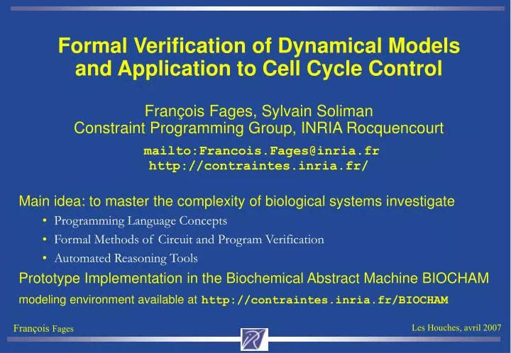
1. Formal Verification of Dynamical Models and Application to Cell Cycle ControlFrançois Fages, Sylvain SolimanConstraint Programming Group, INRIA Rocquencourtmailto:Francois.Fages@inria.frhttp://contraintes.inria.fr/ • Main idea: to master the complexity of biological systems investigate • Programming Language Concepts • Formal Methods of Circuit and Program Verification • Automated Reasoning Tools • Prototype Implementation in the Biochemical Abstract Machine BIOCHAM • modeling environment available athttp://contraintes.inria.fr/BIOCHAM

2. Systems Biology • “Systems Biology aims at systems-level understanding [which] • requires a set of principles and methodologies that links the • behaviors of molecules to systems characteristics and functions.” • H. Kitano, ICSB 2000 • Analyze (post-)genomic data produced with high-throughput technologies (stored in databases like GO, KEGG, BioCyc, etc.); • Integrate heterogeneous data about a specific problem; • Understand and Predict behaviors or interactions in big networks of genes or proteins. • Systems Biology Markup Language (SBML) : exchange format for reaction models

3. Issue of Abstraction • Models are built in Systems Biology with two contradictory perspectives :

4. Issue of Abstraction • Models are built in Systems Biology with two contradictory perspectives : • 1) Models for representing knowledge : the more concrete the better

5. Issue of Abstraction • Models are built in Systems Biology with two contradictory perspectives : • 1) Models for representing knowledge : the more concrete the better • 2) Models for making predictions : the more abstract the better !

6. Issue of Abstraction • Models are built in Systems Biology with two contradictory perspectives : • 1) Models for representing knowledge : the more concrete the better • 2) Models for making predictions : the more abstract the better ! • These perspectives can be reconciled by organizing formalisms and models into hierarchies of abstractions. • To understand a system is not to know everything about it but to know • abstraction levels that are sufficient for answering questions about it

7. Language-based Approaches to Cell Systems Biology • Qualitative models:from diagrammatic notation to • Boolean networks [Kaufman 69, Thomas 73] Petri Nets [Reddy 93, Chaouiya 05] • Process algebra π–calculus[Regev-Silverman-Shapiro 99-01, Nagasali et al. 00] • Bio-ambients [Regev-Panina-Silverman-Cardelli-Shapiro 03] • Pathway logic [Eker-Knapp-Laderoute-Lincoln-Meseguer-Sonmez 02] • Reaction rules[Chabrier-Fages 03] [Chabrier-Chiaverini-Danos-Fages-Schachter 04] • Quantitative models: from ODEs and stochastic simulations to • Hybrid Petri nets [Hofestadt-Thelen 98, Matsuno et al. 00] • Hybrid automata [Alur et al. 01, Ghosh-Tomlin 01] HCC [Bockmayr-Courtois 01] • Stochastic π–calculus [Priami et al. 03] [Cardelli et al. 06] • Reaction rules with continuous time dynamics[Fages-Soliman-Chabrier 04]

8. Overview of the Lecture • Rule-based Language for Modeling Biochemical Systems • Syntax of molecules, compartments and reactions • Semantics at three abstraction levels: boolean, differential, stochastic • Simple examples of signal transduction, transcription, cell-cell interaction • Temporal Logic Language for Formalizing Biological Properties • CTL for the boolean semantics • Constraint LTL for the differential semantics • PCTL for the stochastic semantics • Automated Reasoning Tools • Inferring kinetic parameter values from Constraint-LTL specification • Inferring reaction rules from CTL specification • Type inference by abstract interpretation • L. Calzone, N. Chabrier, F. Fages, S. Soliman. TCSB VI, LNBI 4220:68-94. 2006.

9. Formal Proteins • Cyclin dependent kinase 1 Cdk1 • (free, inactive) • Complex Cdk1-Cyclin B Cdk1–CycB • (low activity preMPF) • Phosphorylated form Cdk1~{thr161}-CycB • at site threonine 161 • (high activity MPF) [Alberts et al 2002]

10. Syntax of BIOCHAM Objects • E == name | E-E | E~{p1,…,pn}

11. Syntax of BIOCHAM Objects • E == name | E-E | E~{p1,…,pn} • name: molecule, #gene binding site, abstract @process… • - : binding operator for protein complexes, gene bindings, … • Associative and commutative. • ~{…}: modification operator for phosphorylated sites, acetylated, etc… • Set of modified sites (associative, commutative, idempotent).

12. Syntax of BIOCHAM Objects • E == name | E-E | E~{p1,…,pn} • name: molecule, #gene binding site, abstract @process… • - : binding operator for protein complexes, gene bindings, … • Associative and commutative. • ~{…}: modification operator for phosphorylated sites, acetylated, etc… • Set of modified sites (associative, commutative, idempotent). • O == E | E::location • Location: symbolic compartment (nucleus, cytoplasm, cell …)

13. Syntax of BIOCHAM Objects • E == name | E-E | E~{p1,…,pn} • name: molecule, #gene binding site, abstract @process… • - : binding operator for protein complexes, gene bindings, … • Associative and commutative. • ~{…}: modification operator for phosphorylated sites, acetylated, etc… • Set of modified sites (associative, commutative, idempotent). • O == E | E::location • Location: symbolic compartment (nucleus, cytoplasm, cell …) • S == _ | O+S • + : solution multiset operator (associative, commutative, neutral element _)

14. Basic Rule Schemas • Complexation: A + B => A-B Decomplexation A-B => A + B • cdk1+cycB => cdk1–cycB

15. Basic Rule Schemas • Complexation: A + B => A-B Decomplexation A-B => A + B • cdk1+cycB => cdk1–cycB • Phosphorylation: A =[C]=> A~{p} Dephosphorylation A~{p} =[C]=> A • Cdk1-CycB =[Myt1]=> Cdk1~{thr161}-CycB • Cdk1~{thr14,tyr15}-CycB =[Cdc25~{Nterm}]=> Cdk1-CycB

16. Basic Rule Schemas • Complexation: A + B => A-B Decomplexation A-B => A + B • cdk1+cycB => cdk1–cycB • Phosphorylation: A =[C]=> A~{p} Dephosphorylation A~{p} =[C]=> A • Cdk1-CycB =[Myt1]=> Cdk1~{thr161}-CycB • Cdk1~{thr14,tyr15}-CycB =[Cdc25~{Nterm}]=> Cdk1-CycB • Synthesis: _ =[C]=> A. Degradation: A =[C]=> _. • _ =[#Ge2-E2f13-Dp12]=> CycA cycE =[@UbiPro]=> _ • (not for cycE-cdk2 which is stable)

17. Basic Rule Schemas • Complexation: A + B => A-B Decomplexation A-B => A + B • cdk1+cycB => cdk1–cycB • Phosphorylation: A =[C]=> A~{p} Dephosphorylation A~{p} =[C]=> A • Cdk1-CycB =[Myt1]=> Cdk1~{thr161}-CycB • Cdk1~{thr14,tyr15}-CycB =[Cdc25~{Nterm}]=> Cdk1-CycB • Synthesis: _ =[C]=> A. Degradation: A =[C]=> _. • _ =[#Ge2-E2f13-Dp12]=> CycA cycE =[@UbiPro]=> _ • (not for cycE-cdk2 which is stable) • Transport: A::L1 => A::L2 • Cdk1~{p}-CycB::cytoplasm => Cdk1~{p}-CycB::nucleus

18. From Syntax to Semantics • R ::= S=>S

19. From Syntax to Semantics • R ::= S=>S | S =[O]=> S | S <=> S | S <=[O]=> S • where A =[C]=> B stands for A+C => B+C • A <=> B stands for A=>B and B=>A, etc. • | kinetic for R (import/export SBML format)

20. From Syntax to Semantics • R ::= S=>S | S =[O]=> S | S <=> S | S <=[O]=> S • where A =[C]=> B stands for A+C => B+C • A <=> B stands for A=>B and B=>A, etc. • | kinetic for R (import/export SBML format) • In SBML : no semantics (exchange format)

21. From Syntax to Semantics • R ::= S=>S | S =[O]=> S | S <=> S | S <=[O]=> S • where A =[C]=> B stands for A+C => B+C • A <=> B stands for A=>B and B=>A, etc. • | kinetic for R (import/export SBML format) • In SBML : no semantics (exchange format) • In BIOCHAM : three abstraction levels • Boolean Semantics: presence-absence of molecules • Concurrent Transition System (asynchronous, non-deterministic)

22. From Syntax to Semantics • R ::= S=>S | S =[O]=> S | S <=> S | S <=[O]=> S • where A =[C]=> B stands for A+C => B+C • A <=> B stands for A=>B and B=>A, etc. • | kinetic for R (import/export SBML format) • In SBML : no semantics (exchange format) • In BIOCHAM : three abstraction levels • Boolean Semantics: presence-absence of molecules • Concurrent Transition System (asynchronous, non-deterministic) • Differential Semantics: concentration • Ordinary Differential Equations or Hybrid system (deterministic)

23. From Syntax to Semantics • R ::= S=>S | S =[O]=> S | S <=> S | S <=[O]=> S • where A =[C]=> B stands for A+C => B+C • A <=> B stands for A=>B and B=>A, etc. • | kinetic for R (import/export SBML format) • In SBML : no semantics (exchange format) • In BIOCHAM : three abstraction levels • Boolean Semantics: presence-absence of molecules • Concurrent Transition System (asynchronous, non-deterministic) • Differential Semantics: concentration • Ordinary Differential Equations or Hybrid system (deterministic) • Stochastic Semantics: number of molecules • Continuous time Markov chain

24. 1. Differential Semantics • Associates to each molecule its concentration [Ai]= | Ai| / volume ML-1 • volume of diffusion …

25. 1. Differential Semantics • Associates to each molecule its concentration [Ai]= | Ai| / volume ML-1 • volume of compartment • Compiles a set of rules{ ei for Si=>S’I }i=1,…,n (by default ei is MA(1)) • into the system of ODEs (or hybrid automaton) over variables {A1,…,Ak} • dA/dt = Σni=1 ri(A)*ei - Σnj=1 lj(A)*ej • where ri(A) (resp. li(A)) is the stoichiometric coefficient of A in Si (resp. S’i) • multiplied by the volume ratio of the location of A.

26. 1. Differential Semantics • Associates to each molecule its concentration [Ai]= | Ai| / volume ML-1 • volume of compartment • Compiles a set of rules{ ei for Si=>S’I }i=1,…,n (by default ei is MA(1)) • into the system of ODEs (or hybrid automaton) over variables {A1,…,Ak} • dA/dt = Σni=1 ri(A)*ei - Σnj=1 lj(A)*ej • where ri(A) (resp. li(A)) is the stoichiometric coefficient of A in Si (resp. S’i) • multiplied by the volume ratio of the location of A. • volume_ratio (15,n),(1,c). • mRNAcycA::n <=> mRNAcycA::c. • means 15*Vn = Vc and is equivalent to15*mRNAcycA::n <=> mRNAcycA::c.

27. 1. Differential Semantics • Numerical integration • Adaptive step size 4th order Runge-Kutta (can be weak for stiff systems) • Rosenbrock implicit method using the Jacobian matrix ∂x’i/∂xj • computes a (clever) discretization of time and a time series • (t0, X0, dX0/dt), (t1, X1, dX1/dt), …, (tn, Xn, dXn/dt), … • of concentrations and their derivatives at discrete time points

28. 2. Stochastic Semantics • Associates to each molecule its number |Ai| in its location

29. 2. Stochastic Semantics • Associates to each molecule its number |Ai| in its location • Compiles the rule set into a continuous time Markov chain • over vector states (|A1|,…, |Ak|) where the transition rate τi for the reaction ei for Si=>S’I (giving probability after normalization) is

30. 2. Stochastic Semantics • Associates to each molecule its number |Ai| in its location • Compiles the rule set into a continuous time Markov chain • over vector states (|A1|,…, |Ak|) where the transition rate τi for the reaction ei for Si=>S’I (giving probability after normalization) is • [Gillespie 76, Gibson 00] • where Vi is the volume where the reaction occurs and K is Avogadro number • τi = ei for reactions of the form A =>..., • τi = ei /Vi×K for reactions of the form A+B=>..., • τi = 2 × ei /Vi×K for reactions of the form A+A=>...,

31. 2. Stochastic Semantics • Associates to each molecule its number |Ai| in its location • Compiles the rule set into a continuous time Markov chain • over vector states (|A1|,…, |Ak|) where the transition rate τi for the reaction ei for Si=>S’I (giving probability after normalization) is • [Gillespie 76, Gibson 00] • where Vi is the volume where the reaction occurs and K is Avogadro number • τi = ei for reactions of the form A =>..., • τi = ei /Vi×K for reactions of the form A+B=>..., • τi = 2 × ei /Vi×K for reactions of the form A+A=>..., • Computes realizations as time series (t0, X0), (t1, X1), …, (tn, Xn), …

32. 2. Stochastic Semantics • Associates to each molecule its number |Ai| in its location • Compiles the rule set into a continuous time Markov chain • over vector states (|A1|,…, |Ak|) where the transition rate τi for the reaction ei for Si=>S’I (giving probability after normalization) is • [Gillespie 76, Gibson 00] • where Vi is the volume where the reaction occurs and K is Avogadro number • τi = ei for reactions of the form A =>..., • τi = ei /Vi×K for reactions of the form A+B=>..., • τi = 2 × ei /Vi×K for reactions of the form A+A=>..., • The differential semantics is an abstraction of the stochastic one [Gillespie 76]

33. 3. Boolean Semantics • Associates to each molecule a Boolean denoting its presence/absence in its location

34. 3. Boolean Semantics • Associates to each molecule a Boolean denoting its presence/absence in its location • Compiles the rule set into an asynchronous transition system

35. 3. Boolean Semantics • Associates to each molecule a Boolean denoting its presence/absence in its location • Compiles the rule set into an asynchronous transition system where a reaction like A+B=>C+D is translated into 4 transition rules taking into account the possible complete consumption of reactants: • A+BA+B+C+D • A+BA+B +C+D • A+BA+B+C+D • A+BA+B+C+D

36. 3. Boolean Semantics • Associates to each molecule a Boolean denoting its presence/absence in its location • Compiles the rule set into an asynchronous transition system where a reaction like A+B=>C+D is translated into 4 transition rules taking into account the possible complete consumption of reactants: • A+BA+B+C+D • A+BA+B +C+D • A+BA+B+C+D • A+BA+B+C+D • Necessary to over-approximate the possible behaviors under : • the stochastic semantics : trivial abstraction N  {zero, non-zero} • the differential semantics : harder to relate mathematically

37. Hierarchy of Semantics abstraction Boolean model Discrete model Differential model Theory of abstract Interpretation [Cousot Cousot 77] Stochastic model concretization

38. Cell Signaling • Receptors: RTK tyrosine kinase, G-protein coupled, Notch…

39. Cell Signaling • Receptors: RTK tyrosine kinase, G-protein coupled, Notch… • Signals: hormones insulin, adrenaline, steroids, EGF, … membrane proteins Delta, … nutriments, light, pressure …

40. Cell Signaling • Receptors: RTK tyrosine kinase, G-protein coupled, Notch… • Signals: hormones insulin, adrenaline, steroids, EGF, … membrane proteins Delta, … nutriments, light, pressure … L + R <=> L-R

41. Cell Signaling • Receptors: RTK tyrosine kinase, G-protein coupled, Notch… • Signals: hormones insulin, adrenaline, steroids, EGF, … membrane proteins Delta, … nutriments, light, pressure … L + R <=> L-R L-R + L-R <=> L-R-L-R

42. Cell Signaling • Receptors: RTK tyrosine kinase, G-protein coupled, Notch… • Signals: hormones insulin, adrenaline, steroids, EGF, … membrane proteins Delta, … nutriments, light, pressure … L + R <=> L-R L-R + L-R <=> L-R-L-R RAS-GDP =[L-R-L-R]=> RAS-GTP

43. MAPK Signaling Pathways • Input:RAFactivated by the receptor • RAF-p14-3-3 + RAS-GTP => RAF + p14-3-3 + RAS-GDP • Output:MAPK~{T183,Y185} • moves to the nucleus • phosphorylates a transcription factor • which stimulates gene transcription

44. MAPK Signalling Network [Levchencko et al 2000] • (MA(1),MA(0.4)) forRAF + RAFK <=> RAF-RAFK. • MA(0.1) for RAF-RAFK => RAFK + RAF~{p1}.

45. MAPK Signalling Network [Levchencko et al 2000] • (MA(1),MA(0.4)) forRAF + RAFK <=> RAF-RAFK. • MA(0.1) for RAF-RAFK => RAFK + RAF~{p1}. • RAF~{p1} + RAFPH <=> RAF~{p1}-RAFPH. • RAF~{p1}-RAFPH => RAF + RAFPH. • MEK~$P + RAF~{p1} <=> MEK~$P-RAF~{p1} where p2 not in $P. • MEK~{p1}-RAF~{p1} => MEK~{p1,p2} + RAF~{p1}. $P pattern variable for sites or molecules

46. MAPK Signalling Network [Levchencko et al 2000] • (MA(1),MA(0.4)) forRAF + RAFK <=> RAF-RAFK. • MA(0.1) for RAF-RAFK => RAFK + RAF~{p1}. • RAF~{p1} + RAFPH <=> RAF~{p1}-RAFPH. • RAF~{p1}-RAFPH => RAF + RAFPH. • MEK~$P + RAF~{p1} <=> MEK~$P-RAF~{p1} where p2 not in $P. • MEK~{p1}-RAF~{p1} => MEK~{p1,p2} + RAF~{p1}. • MEK-RAF~{p1} => MEK~{p1} + RAF~{p1}. • MEKPH + MEK~{p1}~$P <=> MEK~{p1}~$P-MEKPH. • MEK~{p1}-MEKPH => MEK + MEKPH. • MEK~{p1,p2}-MEKPH => MEK~{p1} + MEKPH. • MAPK~$P+MEK~{p1,p2}<=>MAPK~$P-MEK~{p1,p2} where p2 not in $P. • MAPKPH + MAPK~{p1}~$P <=> MAPK~{p1}~$P-MAPKPH. • MAPK~{p1}-MAPKPH => MAPK + MAPKPH. • MAPK~{p1,p2}-MAPKPH => MAPK~{p1} + MAPKPH. • MAPK-MEK~{p1,p2} => MAPK~{p1} + MEK~{p1,p2}. • MAPK~{p1}-MEK~{p1,p2}=>MAPK~{p1,p2}+MEK~{p1,p2}. $P pattern variable for sites or molecules

47. Bipartite Protein-Reaction Graph of MAPK GraphViz http://www.research.att.co/sw/tools/graphviz

48. Numerical Simulation of MAPK Signaling

49. Boolean Simulation (random) of MAPK Signaling

50. Five MAP Kinase Pathways in Budding Yeast(Saccharomyces Cerevisiae)