Chapter 12

1. Chapter 12 Monopolistic Competition and Oligopoly

2. Topics to be Discussed • Monopolistic Competition • Oligopoly • Price Competition • Competition Versus Collusion: The Prisoners’ Dilemma • Implications of the Prisoners’ Dilemma for Oligopolistic Pricing • Cartels - option Chapter 12

3. Monopolistic Competition • Characteristics • Firms compete by selling differentiated products that are highly substitutable for one another but not perfect substitutes. In other words, the cross-price elasticity of demand are large but not infinite. • Free entry and exit: it is relatively easy for new firms to enter the market with their own brands and for existing firms to leave if their products become unprofitable. Chapter 12

4. Monopolistic Competition • The amount of monopoly power depends on the degree of differentiation. • Examples of this very common market structure include: • Toothpaste • Soap • Cold remedies Chapter 12

5. Monopolistic Competition • Toothpaste • Easy for other firm to introduce new brands of toothpaste ; eg. Colgate • Crest and monopoly power • Procter & Gamble is the sole producer of Crest • Consumers can have a preference for Crest – taste, reputation, decay preventing efficacy • The greater the preference (differentiation) the higher the price. Chapter 12

6. Monopolistic Competition • Two important characteristics • Differentiated but highly substitutable products • Free entry and exit Chapter 12

7. Monopolistic competition face downward sloping of demand curves • They have monopoly power • But that does not mean they have larger profit • Because easy entry and exit – quite similar with perfect competition • The potential to earn profits will attract new firms with competing brands, driving economic profits down to zero. Chapter 12

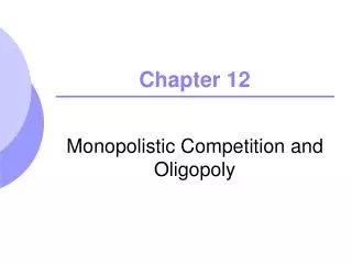
8. MC MC AC AC PSR PLR DSR DLR MRSR MRLR QSR QLR A Monopolistically CompetitiveFirm in the Short and Long Run $/Q $/Q Short Run Long Run Quantity Quantity

9. A Monopolistically CompetitiveFirm in the Short and Long Run • Short-run • Downward sloping demand – differentiated product • Demand is relatively elastic – good substitutes • MR < P • Profits are maximized when MR = MC • This firm is making economic profits Chapter 12

10. A Monopolistically CompetitiveFirm in the Short and Long Run • Long-run • Profits will attract new firms to the industry (no barriers to entry) • The old firm’s demand will decrease to DLR • Firm’s output and price will fall • Industry output will rise • No economic profit (P = AC) • P > MC  some monopoly power Chapter 12

11. Deadweight loss MC AC MC AC P PC D = MR DLR MRLR QC QMC Monopolistically and Perfectly Competitive Equilibrium (LR) Monopolistic Competition Perfect Competition $/Q $/Q P>MC Quantity Quantity

12. Monopolistic Competition & Economic Efficiency • The monopoly power yields a higher price than perfect competition. If price was lowered to the point where MC = D, consumer surplus would increase by the yellow triangle – deadweight loss. • With no economic profits in the long run, the firm is still not producing at minimum AC and excess capacity exists. Chapter 12

13. Monopolistic Competition and Economic Efficiency • Firm faces downward sloping demand so zero profit point is to the left of minimum average cost • Excess capacity is inefficient because average cost would be lower with fewer firms • Inefficiencies would make consumers worse off Chapter 12

14. Monopolistic Competition • If inefficiency bad for consumers, should monopolistic competition be regulated? • Market power relatively small. Usually enough firms to compete with enough substitutability between firms – deadweight loss small • Inefficiency is balance by benefit of increased product diversity – may easily outweigh deadweight loss Chapter 12

15. The Market for Colas and Coffee • Each market has much differentiation in products and try to gain consumers through that differentiation • Coke versus Pepsi • Maxwell House versus Folgers • How much monopoly power do each of these producers have? • How elastic demand for each brand? Chapter 12

16. Elasticities of Demand forBrands of Colas and Coffee Chapter 12

17. The Market for Colas and Coffee • The demand for Royal Crown more price inelastic than for Coke • There is significant monopoly power in these two markets • The greater the elasticity, the less monopoly power and vice versa. Chapter 12

18. Oligopoly – Characteristics • Small number of firms • Product differentiation may or may not exist • Barriers to entry • Scale economies • Patents • Technology • Name recognition • Strategic action Chapter 12

19. Oligopoly • Examples • Automobiles • Steel • Aluminum • Petrochemicals • Electrical equipment Chapter 12

20. Oligopoly • Management Challenges • Strategic actions to deter entry • Threaten to decrease price against new competitors by keeping excess capacity • Rival behavior • Because only a few firms, each must consider how its actions will affect its rivals and in turn how their rivals will react. Chapter 12

21. Oligopoly – Equilibrium • If one firm decides to cut their price, they must consider what the other firms in the industry will do • Could cut price some, the same amount, or more than firm • Could lead to price war and drastic fall in profits for all • Actions and reactions are dynamic, evolving over time Chapter 12

22. Oligopoly – Equilibrium • Defining Equilibrium • Firms are doing the best they can and have no incentive to change their output or price • All firms assume competitors are taking rival decisions into account. • Nash Equilibrium • Each firm is doing the best it can given what its competitors are doing. • We will focus on duopoly • Markets in which two firms compete Chapter 12

23. Oligopoly • The Cournot Model • Oligopoly model in which firms produce a homogeneous good, each firm treats the output of its competitors as fixed, and all firms decide simultaneously how much to produce • Firm will adjust its output based on what it thinks the other firm will produce Chapter 12

24. Firm 1 and market demand curve, D1(0), if Firm 2 produces nothing. D1(0) If Firm 1 thinks Firm 2 will produce 50 units, its demand curve is shifted to the left by this amount. If Firm 1 thinks Firm 2 will produce 75 units, its demand curve is shifted to the left by this amount. MR1(0) D1(75) MR1(75) MC1 MR1(50) D1(50) 12.5 25 50 Firm 1’s Output Decision P1 Q1 Chapter 12

25. Oligopoly • The Reaction Curve • The relationship between a firm’s profit-maximizing output and the amount it thinks its competitor will produce. • A firm’s profit-maximizing output is a decreasing schedule of the expected output of Firm 2. Chapter 12

26. Firm 2’s Reaction Curve Q*2(Q2) Firm 1’s Reaction Curve Q*1(Q2) Reaction Curves and Cournot Equilibrium Q1 Firm 1’s reaction curve shows how much it will produce as a function of how much it thinks Firm 2 will produce. The x’s correspond to the previous model. 100 75 Firm 2’s reaction curve shows how much it will produce as a function of how much it thinks Firm 1 will produce. 50 x x 25 x x Q2 25 50 75 100 Chapter 12

27. Firm 2’s Reaction Curve Q*2(Q2) Cournot Equilibrium Firm 1’s Reaction Curve Q*1(Q2) Reaction Curves and Cournot Equilibrium Q1 100 In Cournot equilibrium, each firm correctly assumes how much its competitors will produce and thereby maximize its own profits. 75 50 x x 25 x x Q2 25 50 75 100 Chapter 12

28. Cournot Equilibrium • Each firms reaction curve tells it how much to produce given the output of its competitor. • Equilibrium in the Cournot model, in which each firm correctly assumes how much its competitor will produce and sets its own production level accordingly. Chapter 12

29. Oligopoly • Cournot equilibrium is an example of a Nash equilibrium (Cournot-Nash Equilibrium) • The Cournot equilibrium says nothing about the dynamics of the adjustment process • Since both firms adjust their output, neither output would be fixed Chapter 12

30. The Linear Demand Curve • An Example of the Cournot Equilibrium • Two firms face linear market demand curve • We can compare competitive equilibrium and the equilibrium resulting from collusion • Market demand is P = 30 - Q • Q is total production of both firms: Q = Q1 + Q2 • Both firms have MC1 = MC2 = 0 Chapter 12

31. Oligopoly Example • Firm 1’s Reaction Curve  MR=MC Chapter 12

32. Oligopoly Example • An Example of the Cournot Equilibrium Chapter 12

33. Oligopoly Example • An Example of the Cournot Equilibrium Chapter 12

34. 30 Firm 2’s Reaction Curve Cournot Equilibrium 15 10 Firm 1’s Reaction Curve 10 15 30 Duopoly Example Q1 The demand curve is P = 30 - Q and both firms have 0 marginal cost. Q2 Chapter 12

35. Oligopoly Example • Profit Maximization with Collusion Chapter 12

36. Profit Maximization w/Collusion • Contract Curve • Q1 + Q2 = 15 • Shows all pairs of output Q1 and Q2 that maximizes total profits • Q1 = Q2 = 7.5 • Less output and higher profits than the Cournot equilibrium Chapter 12

37. Firm 2’s Reaction Curve Competitive Equilibrium (P = MC; Profit = 0) 15 Cournot Equilibrium Collusive Equilibrium 10 7.5 Firm 1’s Reaction Curve Collusion Curve 7.5 10 15 Duopoly Example Q1 For the firm, collusion is the best outcome followed by the Cournot Equilibrium and then the competitive equilibrium 30 Q2 30 Chapter 12

38. First Mover Advantage – The Stackelberg Model • Oligopoly model in which one firm sets its output before other firms do. • Assumptions • One firm can set output first • MC = 0 • Market demand is P = 30 - Q (where Q is total output) • Firm 1 sets output first and Firm 2 then makes an output decision seeing Firm 1 output Chapter 12

39. First Mover Advantage – The Stackelberg Model • Firm 1 • Firm 1 set its output first • Must consider the reaction of Firm 2 • Firm 2 • Firm 2 observe firm 1 then make its output decision • Takes Firm 1’s output as fixed and therefore determines output with the Cournot reaction curve: Q2 = 15 - ½(Q1) Chapter 12

40. First Mover Advantage – The Stackelberg Model • Firm 1 • Choose Q1 so that: • Firm 1 knows firm 2 will choose output based on its reaction curve. WE can use firm 2’s reaction curve as Q2 Recall from previous example Chapter 12

41. First Mover Advantage – The Stackelberg Model • Using Firm 2’s Reaction Curve for Q2: Q2=15-1/2Q1 Chapter 12

42. First Mover Advantage – The Stackelberg Model • Conclusion • Going first gives firm 1 the advantage • Firm 1’s output is twice as large as firm 2’s • Firm 1’s profit is twice as large as firm 2’s • Going first allows firm 1 to produce a large quantity. Firm 2 must take that into account and produce less unless wants to reduce profits for everyone Chapter 12

43. No matter what your competitive does: your output will be large • To maximize profit, your competitor must take your large output level as given and set a low level of output level of output itself • If competitor produced a large level of output, it would drive price down. • Both lose money. Chapter 12

44. The Cournot & Stackelberg models are alternative representations of oligopolistic behavior • Which model is appropriate →depend on industry • Some industry that dominate by a large firm – usually takes the lead in introducing new products or setting price • Eg. The mainframe computer market →IBM the leader • Stackelberg model should be more realistic Chapter 12

45. Price Competition • Competition in an oligopolistic industry may occur with price instead of output. • The Bertrand Model is used • Oligopoly model in which firms produce a homogeneous good • each firm treats the price of its competitors as fixed • and all firms decide simultaneously what price to charge Chapter 12

46. Price Competition – Bertrand Model • Assumptions • Homogenous good • Market demand is P = 30 - Q where Q = Q1 + Q2 • MC1 = MC2 = $3 • Can show the Cournot equilibrium if Q1 = Q2 = 9 and market price is $12 giving each firm a profits of $81. Chapter 12

47. Price Competition – Bertrand Model • Assume here that the firms compete with price, not quantity. • Since good is homogeneous, consumers will buy from lowest price seller • If firms charge different prices, consumers buy from lowest priced firm only • If firms charge same price, consumers are indifferent who they buy from Chapter 12

48. Price Competition – Bertrand Model • Nash equilibrium is competitive output since have incentive to cut prices • Both firms set price equal to MC • P = MC; P1 = P2 = $3 • Q = 27; Q1 & Q2 = 13.5 • Both firms earn zero profit Chapter 12

49. To check whether the outcome is Nash Equilibrium: • Ask whether either firm would have any incentive to change its price • Suppose firm 1 raised its price • It would be lose all of its sales Firm2 • No better off • If lowered the price: capture the entire market but lose money on every unit it produces • No worse off • Firm1 (like Firm 2) has no incentive to deviate • It is going the best it can to maximize profit, given what its competition is doing. Chapter 12

50. Price Competition – Bertrand Model • Why not charge a different price? • If charge more, sell nothing • If charge less, lose money on each unit sold • The Bertrand model demonstrates the importance of the strategic variable • Price versus output Chapter 12