Download
1 / 32
330 likes | 452 Views
Magnetic field and flavor effects on the neutrino fluxes from cosmic accelerators. WIN 2011 January 31-February 5, 2011 Cape Town , South Africa Walter Winter Universität Würzburg. TexPoint fonts used in EMF: A A A A A A A A. Contents. Introduction

E N D
Magnetic field and flavor effects on the neutrino fluxes from cosmic accelerators WIN 2011 January 31-February 5, 2011Cape Town, South Africa Walter Winter Universität Würzburg TexPoint fonts used in EMF: AAAAAAAA
Contents • Introduction • Simulation of sources, a self-consistent approach • Neutrino propagation and detection;flavor ratios • On gamma-ray burst (GRB) neutrino fluxes • Summary
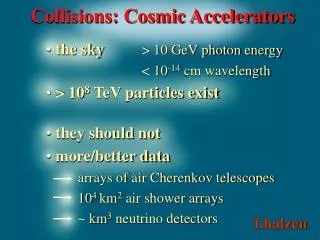
Neutrino production in astrophysical sources max. center-of-mass energy ~ 103 TeV(for 1021 eV protons) Example: Active galaxy(Halzen, Venice 2009)
Neutrino detection: IceCube • Example: IceCube at South PoleDetector material: ~ 1 km3antarctic ice • Completed 2010/11 (86 strings) • Recent data releases, based on parts of the detector: • Point sources IC-40arXiv:1012.2137 • GRB stacking analysis IC-40arXiv:1101.1448 • Cascade detection IC-22arXiv:1101.1692 http://icecube.wisc.edu/
Example: GRB stacking (Source: IceCube) • Idea: Use multi-messenger approach • Predict neutrino flux fromobserved photon fluxesevent by event • Good signal over background ratio (atmospheric background), moderate statistics (Source: NASA) Coincidence! Neutrino observations(e.g. IceCube, …) GRB gamma-ray observations(e.g. Fermi GBM, Swift, etc) (Example: IceCube, arXiv:1101.1448)
IC-40 data meet generic bounds (arXiv:1101.1448) • Generic flux based on the following assumptions:- GRBs are the sources of (highest energetic) cosmic rays- Fraction of energy the protons loose in pion production ~ 20%(Waxman, Bahcall, 1999; Waxman, 2003) What do such bounds actually mean more generically? Limit IC-40 stacking limit Fraction of p energy lost into pion production(related to optical thicknessof pg/ng interactions) Baryonic loading(ratio between protons andelectrons/positrons in the jet) X
When do we expect a n signal?[some personal comments] • Unclear if specific sources lead to neutrino production; spectral energy distribution can be often described by leptonic processes as well (e.g. inverse Compton scattering, …) • However: whereever cosmic rays are produced, neutrinos should be produced as well (pg, pp!) • There are a number of additional candidates, e.g. • „Hidden“ sources (e.g. „slow jet supernovae“ without gamma-ray counterpart)(Razzaque, Meszaros, Waxman, 2004; Ando, Beacom, 2005; Razzaque, Meszaros, 2005; Razzaque, Smirnov, 2009) • Large fraction of Fermi-LAT unidentified sources? • From the neutrino point of view: „Fishing in the dark blue sea“? Looking at the wrong places? • Need for tailor-made neutrino-specific approaches?
Meson photoproduction • Often used: D(1232)-resonance approximation • Limitations: • No p- production; cannot predict p+/ p- ratio (affects neutrino/antineutrino) • High energy processes affect spectral shape • Low energy processes (t-channel) enhance charged pion production • Charged pion production underestimated compared to p0 production by factor of 2.4 (independent of input spectra!) • Solutions: • SOPHIA: most accurate description of physicsMücke, Rachen, Engel, Protheroe, Stanev, 2000Limitations: Often slow, difficult to handle; helicity dep. muon decays! • Parameterizations based on SOPHIA • Kelner, Aharonian, 2008Fast, but no intermediate muons, pions (cooling cannot be included) • Hümmer, Rüger, Spanier, Winter, 2010Fast (~3000 x SOPHIA), including secondaries and accurate p+/ p- ratios; also individual contributions of different processes (allows for comparison with D-resonance!) • Engine of the NeuCosmA („Neutrinos from Cosmic Accelerators“) software from:Hümmer, Rüger, Spanier, Winter, ApJ 721 (2010) 630 T=10 eV
NeuCosmA key ingredients(„Neutrinos from Cosmic Accelerators“) • What it can do so far: • Photohadronics based on SOPHIA(Hümmer, Rüger, Spanier, Winter, 2010) • Weak decays incl. helicity dependence of muons(Lipari, Lusignoli, Meloni, 2007) • Cooling and escape • Potential applications: • Parameter space studies • Flavor ratio predictions • Time-dependent AGN simulations etc. (photohadronics) • Monte Carlo sampling of diffuse fluxes • Stacking analysis with measured target photon fields • Fits (need accurate description!) • … Kinematics ofweak decays: muon helicity! from: Hümmer, Rüger, Spanier, Winter, ApJ 721 (2010) 630
A self-consistent approach • Target photon field typically: • Put in by hand (e.g. obs. spectrum: GRBs) • Thermal target photon field • From synchrotron radiation of co-accelerated electrons/positrons (AGN-like) • Requires few model parameters, mainly • Purpose: describe wide parameter ranges with a simple model; minimal set of assumptions for n!? ?
Model summary Dashed arrows: include cooling and escape Dashed arrow: Steady stateBalances injection with energy losses and escapeQ(E) [GeV-1 cm-3 s-1] per time frameN(E) [GeV-1 cm-3] steady spectrum Opticallythinto neutrons Injection Energy losses Escape Hümmer, Maltoni, Winter, Yaguna, Astropart. Phys. 34 (2010) 205
An example (1) a=2, B=103 G, R=109.6 km • Meson production described by(summed over a number of interaction types) • Only product normalization enters in pion spectra as long as synchrotron or adiabatic cooling dominate • Maximal energy of primaries (e, p) by balancing energy loss and acceleration rate Maximum energy: e, p Hümmer, Maltoni, Winter, Yaguna, 2010
An example (2) a=2, B=103 G, R=109.6 km • Secondary spectra (m, p, K) become loss-steepend above a critical energy • Ec depends on particle physics only (m, t0), and B • Leads to characteristic flavor composition • Any additional cooling processes mainly affecting the primaries will not affect the flavor composition • Flavor ratios most robust predicition for sources? Cooling: charged m, p, K Ec Ec Ec Hümmer, Maltoni, Winter, Yaguna, 2010
An example (3) a=2, B=103 G, R=109.6 km m cooling break Synchrotroncooling Spectralsplit p cooling break Pile-up effect Flavor ratio! Pile-upeffect Slope:a/2 Hümmer, Maltoni, Winter, Yaguna, 2010
The Hillas plot • Hillas (necessary) condition for highest energetic cosmic rays (h: acc. eff.) • Protons, 1020 eV, h=1: • We interpret R and B as parameters in bulk frame • High bulk Lorentz factors G relax this condition! Hillas 1984; version adopted from M. Boratav
Flavor composition at the source(Idealized – energy independent) • Astrophysical neutrino sources producecertain flavor ratios of neutrinos (ne:nm:nt): • Pion beam source (1:2:0)Standard in generic models • Muon damped source (0:1:0)at high E: Muons loose energy before they decay • Muon beam source (1:1:0)Cooled muons pile up at lower energies (also: heavy flavor decays) • Neutron beam source (1:0:0)Neutron decays from pg(also possible: photo-dissociationof heavy nuclei) • At the source: Use ratio ne/nm (nus+antinus added)
However: flavor composition is energy dependent! Pion beam Muon beam muon damped Energywindowwith largeflux for classification Typicallyn beamfor low E(from pg) Pion beam muon damped Undefined(mixed source) Behaviorfor smallfluxes undefined (from Hümmer, Maltoni, Winter, Yaguna, 2010; see also: Kashti, Waxman, 2005; Kachelriess, Tomas, 2006, 2007; Lipari et al, 2007)
Parameter space scan • All relevant regions recovered • GRBs: in our model a=4 to reproduce pion spectra; pion beam muon damped (confirmsKashti, Waxman, 2005) • Some dependence on injection index a=2 Hümmer, Maltoni, Winter, Yaguna, 2010
Neutrino propagation • Key assumption: Incoherent propagation of neutrinos • Flavor mixing: • Example: For q13 =0, q12=p/6, q23=p/4: • NB: No CPV in flavor mixing only!But: In principle, sensitive to Re exp(-i d) ~ cosd • Take into account Earth attenuation! (see Pakvasa review, arXiv:0803.1701, and references therein)
Which sources can specific data constrain best? • Constrain individual fluxes after flavor mixing with existing data Point sources IC-40arXiv:1012.2137 Energy flux density PRELIMINARY (work in preparation)
Measuring flavor? • In principle, flavor information can be obtained from different event topologies: • Muon tracks - nm • Cascades (showers) – CC: ne, nt, NC: all flavors • Glashow resonance: ne • Double bang/lollipop: nt (Learned, Pakvasa, 1995; Beacom et al, 2003) • In practice, the first (?) IceCube „flavor“ analysis appeared recently – IC-22 cascades (arXiv:1101.1692)Flavor contributions to cascades for E-2 extragalatic test flux (after cuts): • Electron neutrinos 40% • Tau neutrinos 45% • Muon neutrinos 15% • Electron and tau neutrinos detected with comparable efficiencies • Neutral current showers are a moderate background t nt
Flavor ratios at detector • At the detector: define observables which • take into account the unknown flux normalization • take into account the detector properties • Example: Muon tracks to showersDo not need to differentiate between electromagnetic and hadronic showers! • Flavor ratios have recently been discussed for many particle physics applications (for flavor mixing and decay: Beacom et al 2002+2003; Farzan and Smirnov, 2002; Kachelriess, Serpico, 2005; Bhattacharjee, Gupta, 2005; Serpico, 2006; Winter, 2006; Majumar and Ghosal, 2006; Rodejohann, 2006; Xing, 2006; Meloni, Ohlsson, 2006; Blum, Nir, Waxman, 2007; Majumar, 2007; Awasthi, Choubey, 2007; Hwang, Siyeon,2007; Lipari, Lusignoli, Meloni, 2007; Pakvasa, Rodejohann, Weiler, 2007; Quigg, 2008; Maltoni, Winter, 2008; Donini, Yasuda, 2008; Choubey, Niro, Rodejohann, 2008; Xing, Zhou, 2008; Choubey, Rodejohann, 2009; Esmaili, Farzan, 2009; Bustamante, Gago, Pena-Garay, 2010; Mehta, Winter, 2011…)
Parameter uncertainties • Basic dependencerecovered afterflavor mixing • However: mixing parameter knowledge ~ 2015 (Daya Bay, T2K, etc) required Hümmer, Maltoni, Winter, Yaguna, 2010
New physics in R? Energy dependenceflavor comp. source Energy dep.new physics (Example: [invisible] neutrino decay) 1 Stable state 1 Unstable state Mehta, Winter, arXiv:1101.2673
Which sources are most useful? • Most useful:Sources for which different flavor compositions are present; requires substantial B • Some dependence on new physics effect aL=108 GeV No of decayscenarios which canbe identified Mehta, Winter, arXiv:1101.2673
Waxman-Bahcall, reproduced • Difference to above: target photon field ~ observed photon field used • Reproduced original WB flux with similar assumptions • Additional charged pion production channels included,also p-! broken power law(Band function) p decays only ~ factor 6 Baerwald, Hümmer, Winter, arXiv:1009.4010
Fluxes before flavor mixing ne nm Baerwald, Hümmer, Winter, arXiv:1009.4010
After flavor mixing Consequences: • Different flux shape • Can double peak structure be used? • How reliable is stacking analysis from IC-40? • Different normalization • Expect actually more neutrinos than in original estimates • Baryonic loading x fpstronger constrained? • GRBs not the sourcesof highest energetic CR? (full scale) (full scale) Baerwald, Hümmer, Winter, arXiv:1009.4010; see also: Murase, Nagataki, 2005; Kashti, Waxman, 2005; Lipari, Lusignoli, Meloni, 2007
Summary • Particle production, flavor, and magnetic field effects change the shape of astrophysical neutrino fluxes • Description of the „known“ (particle physics) components should be as accurate as possible for data analysis • Flavor ratios, though difficult to measure, are interesting because • they may be the only way to directly measure B (astrophysics) • they are useful for new physics searches (particle physics) • they are relatively robust with respect to the cooling and escape processes of the primaries (e, p, g) • However: flavor ratios should be interpreted as energy-dependent quantities • The flux shape and flavor ratio of a point source can be predicted in a self-consistent way if the astrophysical parameters can be estimated, such as from a multi-messenger observation (R: from time variability, B: from energy equipartition, a: from spectral shape)