Global Illumination

1. Global Illumination

2. Direct Illumination vs. Global Illumination reflected, scattered and focused light (not discreet). physical-based light transport calculations modeled around bidirectional reflective distribution functions (BRDFs). discreet light source. efficient lighting calculations based on light and surface vectors (i.e. fast cheats).

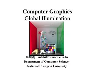
3. Indirect Illumination Color Bleeding

4. Contact Shadows Notice the surface just under the sphere. The shadow gets much darker where the direct illumination as well as most of the indirect illumination is occluded. That dark contact shadow helps enormously in “sitting” the sphere in scene. Contact shadows are difficult to fake, even with area lights.

5. Caustics • Focused and reflected light, or caustics, are another feature of the real world that we lack in direct illumination.

6. Global illumination rendered images Caustics are a striking and unique feature of Global Illumination.

7. BRDF • BRDF really just means “the way light bounces off of something.” • Specular reflection: some of the light bounces right off of the surface along the angle of reflection without really changing color much. • Diffuse reflection: some of the light gets refracted into the plastic and bounced around between red particles of pigment. Most of the green and the blue light is absorbed and only the red light makes it’s way back out of the surface. The red light bounced back is scattered every which way with fairly equal probability.

8. Rendering Equation • L is the radiance from a point on a surface in a given direction ω • E is the emitted radiance from a point: E is non-zero only if x’ is emissive • V is the visibility term: 1 when the surfaces are unobstructed along the direction ω, 0 otherwise • G is the geometry term, which depends on the geometric relationship between the two surfaces x and x’ • It includes contributions from light bounded many times off surfaces • f is the BRDF

9. Light Emitted from a Surface • Radiance (L): Power per unit area per unit solid angle • Measured in W/m2sr • dA is projected area – perpendicular to given direction • Radiosity (B): Radiance integrated over all directions • Power from per unit area, measured in W/m2

10. Radiosity Concept • Radiosity of each surface depends on radiosity of all other surfaces • Treat global illumination as a linear system • Need constant BRDF (diffuse) • Solve rendering equation as a matrix problem • Process • Mesh into patches • Calculate form factors • Solve radiosity • Display patches Cornell Program of Computer Graphics

11. Radiosity Equation Assume only diffuse reflection Convert to radiosity

12. Radiosity Approximations Discretize the surface into patches The form factor Fii = 0 (patches are flat) Fij = 0 if occluded Fij is dimensionless

13. Radiosity Matrix Such an equation exists for each patch, and in a closed environment, a set of n Simultaneous equations in n unknown Bi values is obtained: A solution yields a single radiosity value Bi for each patch in the environment – a view-independent solution. The Bi values can be used in a standard renderer and a particular view of the environment constructed from the radiosity solution.

14. Intuition

15. Form Factor Intuition

16. Hemicube • Compute form factor with image-space precision • Render scene from centroid of Ai • Use z-buffer to determine visibility of other surfaces • Count “pixels” to determine projected areas

17. Monte Carlo Sampling • Compute form factor by random sampling • Select random points on elements • Intersect line segment to evaluate Vij • Evaluate Fij by Monte Carlo integration

18. Solving the Radiosity Equations • Solution methods: • Invert the matrix – O(n3) • Iterative methods – O(n2) • Hierarchical methods – O(n)

19. Examples Museum simulation. Program of Computer Graphics, Cornell University. 50,000 patches. Note indirect lighting from ceiling.

20. Gauss-Siedel Iteration method • For all i Bi = Ei • While not converged For each i in turn • Display the image using Bi as the intensity of patch i

21. Interpretation of Iteration • Iteratively gather radiosity to elements

22. Progressive Radiosity

23. Progressive Radiosity • Interpretation: • Iteratively shoot “unshot” radiosity from elements • Select shooters in order of unshot radiosity

24. Progressive Radiosity

25. Adaptive Meshing • Refine mesh in areas of large errors

26. Adaptive Meshing Uniform Meshing Adaptive Meshing

27. Hierarchical Radiosity • Refine elements hierarchically: • Compute energy exchange at different element granularity • satisfying a user-specified error tolerance

28. Hierarchical Radiosity

29. Hierarchical Radiosity

30. Displaying Radiosity Usually Gouraud Shading Computed Rendered

31. Radiosity • Constrained by the resolution of your subdivision patches. • Have to calculate all of the geometry before you rendered an image. • No reflections or specular component.

32. Path Types • OpenGL • L(D|S)E • Ray Tracing • LDS*E • Radiosity • LD*E • Path Tracing • attempts to trace“all rays” in a scene

33. objects lights Ray Tracing • LDS*E Paths • Rays cast from eye into scene Why? Because most rays cast from light wouldn’t reach eye • Shadow rays cast at each intersection Why? Because most rays wouldn’t reach the light source • Workload badly distributed Why? Because # of rays grows exponentially, and their result becomes less influential

34. Tough Cases • Caustics • Light focuses through a specular surface onto a diffuse surface • LSDE • Which direction should secondary rays be cast to detect caustic? • Bleeding • Color of diffuse surface reflected in another diffuse surface • LDDE • Which direction should secondary rays be cast to detect bleeding?

35. objects lights Path Tracing • Kajiya, SIGGRAPH 86 • Diffuse reflection spawns infinite rays • Pick one ray at random • Cuts a path through the dense ray tree • Still cast an extra shadow ray toward light source at each step in path • Trace > 40 paths per pixel

36. Monte Carlo Path Tracing • Integrate radiance for each pixel by sampling paths randomly

37. Basic Monte Carlo Path Tracer • Choose a ray (x, y), t; weight = 1 • race ray to find intersection with nearest surface • Randomly decide whether to compute emitted or reflected light • Step 3a: If emitted, return weight * Le • Step 3b: If reflected, weight *= reflectance Generate ray in random direction Go to step 2

38. Bi-directional Path Tracing • Role of source and receiver can be switched, flux does not change

39. Bi-directional Path Tracing

40. Tracing from eye

41. Tracing from light

42. Monte Carlo Path Tracing • Advantages • Any type of geometry (procedural, curved, ...) • Any type of BRDF (specular, glossy, diffuse, ...) • Samples all types of paths (L(SD)*E) • Accurate control at pixel level • Low memory consumption • Disadvantages • Slow convergence • Noise in the final image

43. Monte Carlo path tracing 1000 path / pixel

44. Monte Carlo Ray Tracing It’s worse when you have small light sources (e.g. the sun) or lots of light and dark variation (i.e. high-frequency) in your environment.

45. Monte Carlo Integration That’s why you always see “overcast” lighting like this.

46. Noise Filtering filtered Unfiltered van Jensen, Stanford

47. Photon Mapping • Monte Carlo path tracing relies on lots of camera rays to “find” the bright areas in a scene. Small bright areas can be a real problem. (Hence the typical “overcast” lighting). • Why not start from the light sources themselves, scatter light into the environment, and keep track of where the light goes?

48. Photon Mapping • Jensen EGRW 95, 96 • Simulates the transport of individual photons • Photons emitted from source • Photons deposited on diffuse surfaces • Photons reflected from surfaces to other surfaces • Photons collected by rendering

49. wp DFp xp What is a Photon? • A photon p is a particle of light that carries flux DFp(xp, wp) • Power: DFp – magnitude (in Watts) and color of the flux it carries, stored as an RGB triple • Position: xp – location of the photon • Direction: wp – the incident direction wi used to compute irradiance • Photons vs. rays • Photons propagate flux • Rays gather radiance

50. Sources • Point source • Photons emitted uniformly in all directions • Power of source (W) distributed evenly among photons • Flux of each photon equal to source power divided by total # of photons • For example, a 60W light bulb would send out a total of 100K photons, each carrying a flux DF of 0.6 mW • Photons sent out once per simulation, not continuously as in radiosity