Download
1 / 51
510 likes | 684 Views
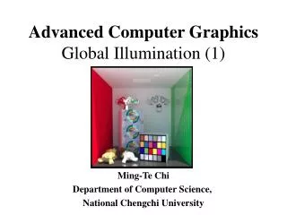
Advanced Global Illumination. Brian Chen Thursday, February 12, 2004. Global Illumination. Physical Simulation of Light Transport: Accuracy account for ALL light paths conservation of energy Prediction forward rendering calculate light meter readings

E N D
Advanced Global Illumination Brian Chen Thursday, February 12, 2004
Global Illumination • Physical Simulation of Light Transport: • Accuracyaccount for ALL light pathsconservation of energy • Predictionforward renderingcalculate light meter readings • Analysisinverse rendering! find surface properties ! • Realism?perceptually necessary?
Global Illumination • “Everything is lit by Everything Else” • Screen color = entire scene’s lighting * surface reflectance • Refinements: Models of area light sources, caustics, soft-shadowing, fog/smoke, photometric calibration, … H. Rushmeier et al., SIGGRAPH`98 Course 05 “A Basic Guide to Global Illumination”
Overview • Physics (Optics) concepts • Models of Light • Radiometry • BRDFs & Rendering Equation • Monte Carlo Methods • Photon Mapping
Optics Definitions • Reflection – when light bounces off a surface • Refraction – the bending of light when it goes through different mediums (ex. air and glass) • Diffraction – the phenomenon where light “bends” around obstructing objects • Dispersion – when white light splits into its components colors, result of refraction
Light’s Dual Nature • Is light a wave? Or is it a beam of particles? • Wave Theory of Light – Thomas Young’s double-slit experiment • Particle Theory of Light – Newton, refraction & dispersion
Light Models • Models of light are used to capture/explain the different behaviors of light that stem from its dual nature • Quantum Optics • Wave Model • Geometric Optics
Quantum Optics • Explains dual wave-particle nature at the submicroscopic level of electrons • Way too detailed for purposes of image generation for computer graphics scenes • Therefore, it is not used
Wave Model • Simplification of Quantum Model • Captures effects that occur when light interacts with objects of size comparable to the wavelength of light (diffraction, polarization) • This model is also ignored, too complex and detailed
Geometric Optics • Simplest and most commonly used light model • Assumes light is emitted, reflected, and transmitted (refraction) • Also assumes: • Light travels in straight lines, no diffraction • Light travels instantaneously through a medium (travels at infinite speed) • Light is not influenced by gravity, magnetic fields
Radiometry • Radiometry – area of study involved in the physical measurement of light • Goal of illumination algorithm is to compute the steady-state distribution of light energy in a scene
Radiometric Quantities • Radiant Power • flux (in Watts = Joule/sec), Φ • How much total energy flows from/to/through a surface per unit time • Irradiance (“ear”) • incoming radiant power on a surface per unit surface area (Watt/m2) • E = dΦ/dA
More Radiometric Quantities • Radiosity • Outgoing radiant power per unit surface area (Watt/m2) • B = dΦ/dA
Radiance • Flux per unit projected area per unit solid angle (W/(steradian x m2)) • How much power arrives at (or leaves from) a certain point on a surface, per unit solid angle, and per unit projected area • L(x, Ө) = d2Φ / (dω dA cosӨ) • The most important quantity in global illumination because it captures the “appearance” of objects
Radiance cont’d Radiance: The Pointwise Measure of Light • Free-space light power L ==(energy/time) • At least a 5D scalar function:L(x, y, z, , , …) • Position (x,y,z), Angle (,) and more (t, , …) • Power density units, but tricky… Taken with permission from Jack Tumblin
Yet More Radiance Tricky: think Hemispheres with a floor: Solid Angle (steradians) =dω = fraction of a hemisphere’s area (4) Projected Area cos dA dA Taken with permission from Jack Tumblin
Properties of Radiance • 1: Radiance is invariant along straight paths and does not attenuate with distance • Radiance leaving point x directed towards point y is equal to the radiance arriving at point y from the point x • 2: Sensors, such as cameras and human eye, are sensitive to radiance • The response of our eyes is proportional to the radiance incident upon them. • It is now clear that radiance is the quantity that global illumination algorithms must compute and display to the observer
BRDF (Bidirectional Reflectance Distribution Function) • Intuitively the BRDF represents, for each incoming angle, the amount of light that is scattered in each outgoing angle • BRDF at a point x is defined as the ratio of the radiance reflected in an exitant direction (Ө), and the irradiance incident in a differential solid angle (Ψ). • fr(x,Ψ->Ө) = dL(x->Ө) / (L(x<-Ψ)cos(Nx,Ψ)dωΨ) • cos(Nx,Ψ) = cos of angle formed by normal & incident direction vector
Point-wise Reflectance: BRDF Bidirectional Reflectance Distribution Function (i , i , r , r , i , r , …) == (Lr / Li) a scalar (sr-1) Illuminant Li Reflected Lr Infinitesimal Solid Angle
BRDF Properties • Value of BRDF remains unchanged if the incident and outgoing directions are interchanged • Law of conservation of energy requires that the total amount of power reflected all directions must be less than or equal to the total amount of power incident on the surface
BRDF Examples, Diffuse Fr = (x,Ψ<->Ө) = ρd/π, constant ρd is the fraction of incident energy that is reflected at a surface, 0-1 Andrew Glassner et al.. SIGGRAPH`94 Course 18: “Fundamentals and Overview of Computer Graphics”
BRDF Examples, Specular Exitant direction: R = 2(N dot Ψ)N – Ψ Andrew Glassner et al.. SIGGRAPH`94 Course 18: “Fundamentals and Overview of Computer Graphics”
For Most Surfaces Most Materials: Combination of Diffuse & Specular…their BRDF is difficult to model with formulas Andrew Glassner et al.. SIGGRAPH`94 Course 18: “Fundamentals and Overview of Computer Graphics”
Practical Shading Models (BRDF) • Lambert: kd = ρd/π • Phong: fr = ks*((R·Өn)/(N·Ψ)) + kd • Blinn-Phong = ks*((N·H)/(N·Ψ)) + kd, H=halfway vector between Ψ & Ө • Modified Blinn-Phong = ks*(N·H)n + kd • Cook-Torrance • Ward
Rendering Equation Finally! Putting radiance and the BRDF together to get:
BRDF & Rendering Eq. • For example, suppose that we wish to determine the illumination of a scene containing n light sources – light source 1 to light source n. In this case, the local illumination of a surface is given by, • where Lij is the intensity of the jth light source and wij = (ij,ij) is the direction to the jth light source.
BRDF & Rendering Eq. • For a single point light source, the light reflected in the direction of an observer is • This is the general BRDF lighting equation for a single point light source
Rendering Equation Opportunities • Scalar operations only: () and L(), indep. of , x,y,z, , … • Linearity: • Solution = weighted sum of one-light solns. • Many BRDFs weighted sum of diffuse, specular, gloss terms Difficulties • Almost no nontrivial analytic solutions exist; MUST use approximate methods to solve • Verification: tough to measure real-world () and L() well • Notable wavelength-dependent surfaces exist (iridescent insect wings & casing, CD grooves, oil) • BRDF doesn’t capture important subsurface scattering
Review 1 Big Ideas: • Measure Light:Radiance • Measure Light Attenuation: BRDF • Light will ‘bounce around’ endlessly, decaying on each bounce:The Rendering Equation (intractable: must approximate)
Monte Carlo Techniques • Mathematical techniques that use statistical sampling to simulate phenomena or evaluate values of functions • Use a probability distribution function (PDF) to generate random samples, p(x)
Estimators • Unbiased – when the expected value of the estimator is exactly the value of the integral • Biased – when the above property is not true • Bias – the difference between the expected value of the estimator and the actual value of the integral • As number of samples N increases, the estimate becomes closer
Monte Carlo Techniques • The reliability of Monte-Carlo sampling is measured by the variance of the estimators. The variance of the estimators is given as • where is the primary estimator, while its average is a secondary estimator
Monte Carlo Techniques • As a consequence of the above formula, the Monte-Carlo technique requires a large number of samples to reduce the variance of the primary estimator • The error of the approximation is itself a random variable with zero mean, i.e. the estimator is unbiased. The standard deviation of this estimator is reduced only proportional to which is known as the diminishing return of the Monte-Carlo technique, i.e. the number of samples must be quadrupled to reduce the standard deviation by one half.
Monte Carlo Techniques • For importance sampling we adjust the pdf p to be similar in shape to the integrand f. If we were able to choose p(x)= Cf(x), with a constant factor C= 1/I, the variance of the primary estimator would be zero and a single sample would always give the correct result. • Unfortunately, the constant C is determined by the integral we want to compute and is therefore unavailable. On the other hand, some a priori knowledge about the shape of f is often available and can be used to adjust p to reduce the variance of the estimators.
Monte Carlo Example • Computing a one-dimensional integral • Samples are selected randomly over the domain of the integral to get a close approximation (estimator <I> • <I> = (1/N) Σ f(xi) / p(xi)
Another Example • Integration over a hemisphere • Estimate the radiance at a point by integrating the contribution of light sources in the scene • Light source L • I = ∫Lsourcecosdω = ∫02π ∫0 π/2 Lsourcecossinddφ • <I>=(1/N)Σ (Lsource(ωi) cossin) / p(ωi) • p(ωi) = cossin/ π • <I>=(1/N)Σ Lsource(ωi)
Steps • General: • Sampling according to a probability distribution function • Evaluation of the function at that sample • Averaging these appropriately weighted sampled values • Graphics: • Generate random photon paths from source (lights or pixels) • Set a discrete random length for the path • Count how many photons terminate in state i, average radiances for that point
http://graphics.stanford.edu/courses/cs348b-02/lectures/lecture15/walk014.htmlhttp://graphics.stanford.edu/courses/cs348b-02/lectures/lecture15/walk014.html
http://graphics.stanford.edu/courses/cs348b-02/lectures/lecture15/walk014.htmlhttp://graphics.stanford.edu/courses/cs348b-02/lectures/lecture15/walk014.html
Advantages/Disadvantages • Advantages • Simple: just sample signal/function and average estimates • Widely applicable: nuclear physics, graphics, high-dimensional integrations of complicated functions • Can be used with radiosity • Disadvantages • Very slow, take many, many samples to converge to correct solution • Need 4x samples to decrease error by half
Photon Mapping • One of the “fastest” algorithms available for global illumination • Monte-Carlo based • 2-pass algorithm
Photon Mapping, 1st pass • 1st pass • photons shot from the light into the scene • they bounce around interacting with all the types of surfaces they encounter • Clever twists • 1st, instead of redoing those same computations over and over, a few thousand of time for each pixels, the photons are stored only once in a special data structure called a photon map for later reuse • 2nd, instead of trying to completely fill the whole scene with billions of photons, a few thousands to a million photons are sparsely stored and the rest is statistically estimated from the density of the stored photons. • After all the photons have been stored in the map, a statistical estimate of the irradiance at each photon position is computed.
Photon Mapping, 2nd Pass • Direct illumination is computed just like regular ray tracing, but the indirect illumination, which comes from the walls and other objects around, is computed from querying the stored photons in the photon map • At each secondary hit, the photon map is queried in order to gather the radiance coming from the objects around in the environment.