Chapter 4 Advanced Pipelining and Intruction-Level Parallelism
190 likes | 421 Views
Chapter 4 Advanced Pipelining and Intruction-Level Parallelism. Computer Architecture A Quantitative Approach John L Hennessy & David A Patterson 2 nd Edition , 1996, Morgan Kaufmann. Technique Reduces Loop unrolling => Control stalls Basic pipeline scheduling => RAW stalls

Chapter 4 Advanced Pipelining and Intruction-Level Parallelism
E N D
Presentation Transcript
Chapter 4Advanced Pipelining and Intruction-Level Parallelism Computer Architecture A Quantitative Approach John L Hennessy & David A Patterson 2nd Edition , 1996, Morgan Kaufmann
Technique Reduces • Loop unrolling => Control stalls • Basic pipeline scheduling => RAW stalls • Dynamic scheduling with scoreboarding => RAW stalls • Dynamic scheduling with register renaming => WAR & WAW stalls • Dynamic branch prediction => Control stalls • Issuing multiple instructions per cycle => Ideal CPI • Compiler dependence analysis => Ideal CPI & data stalls • Software pipelining and trace scheduling => Ideal CPI & data stalls • Speculation => All data & control stalls • Dynamic memory disambiguation => RAW stalls involving memory
Instruction-Level Parallelism The simplest and most common way to increase the amount of parallelism available among instructions is to exploit parallelism among iterations of a loop. This type of parallelism is often called loop-level parallelism. Here is a simple example of a loop, which adds two 1000-element arrays, that is comletely parallel : for ( i = 1; i <= 1000; i = i + 1 ) x[i] = x[i] + y[i] Every iteration of the loop can overlap with any other iteration, although within each loop iteration there is little opportunity for overlap.
Instruction-Level Parallelism Two strategies to support ILP: • Dynamic Scheduling: depend on the hardware to locate parallelism • Static Scheduling: rely on software for identifying potential parallelism
Basic Pipeline Scheduling and Loop Unrolling for (i = 1; i <= 1000; i++) x[i] = x[i] + s; • Loop : LD F0,0(R1) ; F0 = array element • ADDD F4,F0,F2 ; add scalar in F2 • SD 0(R1),F4 ; store result • SUBI R1,R1,#8 ; decrement pointer 8 bytes • BNEZ R1,Loop ; branch R1 != zero
Without any scheduling : Loop : LD F0,0(R1) 1 stall 2 ADDD F4,F0,F2 3 stall 4 stall 5 SD 0(R1),F4 6 SUBI R1,R1,#8 7 stall 8 BNEZ R1,Loop 9 stall 10 We can schedule the loop to obtain only one stall :Loop : LD F0,0(R1) SUBI R1,R1,#8 ADDD F4,F0,F2 stall BNEZ R1,Loop ; delayed branch SD 8(R1),F4 ; altered & interchanged with SUBIExecution time has been reduced from 10 clock cycles to 6.
In the above example, we complete one loop iteration and store back one array element every 6 clock cycles, but the actual work of operating on the array element takes just 3 (the load, add, and store) of those 6 clock cycles. The remaining 3 clock cycles consist of loop overhead—the SUBI and BNEZ—and a stall. To eliminate these 3 clock cycles we need to get more operations within the loop relative to the number of overhead instructions. A simple scheme for increasing the number of instructions relative to the branch and overhead instructions is loop unrolling. Unrolling simply replicates the loop body multiple times, adjusting the loop termination code.
EXAMPLE Show our loop unrolled so that there are four copies of the loop body, Assuming R1 is initially a multiple of 32, which means that the number of loop iterations is a multiple of 4. Eliminate any obviously redundant computations and do not reuse any of the registers. ANSWER Here is the result after merging the SUBI instructions and dropping the Unnecessary BNEZ operations that are duplicated during unrolling. Note that R2 must now be set so that 32(R2) is the starting address of the last four elements. Loop: LD F0,0(R1) ADDD F4,F0,F2 SD F4,0(R1) ;drop SUBI & BNEZ LD F6,-8(R1) ADDD F8,F6,F2 SD F8,-8(R1) ;drop SUBI & BNEZ LD F10,-16(R1)
ADDD F12,F10,F2 SD F12,-16(R1) ;drop SUBI & BNEZ LD F14,-24(R1) ADDD F16,F14,F2 SD F16,-24(R1) SUBI R1,R1,#-32 BNEZ R1,R2,Loop We have eliminated three branches and three decrements of R1. The addresses on the loads and stores have been compensated to allow the SUBI instructions on R1 to be merged. Without scheduling, every operation in the unrolled loop is followed by a dependent operation and thus will cause a stall. This loop will run in 28 clock cycles—each LD has 1 stall, each ADDD 2, the SUBI 1, the branch 1, plus 14 instruction issue cycles—or 7 clock cycles for each of the four elements. Although this unrolled version is currently slower than the scheduled version of the original loop, this will change when we schedule the unrolled loop. Loop unrolling is normally done early in the compilation process, so that redundant computations can be exposed and eliminated by the optimizer.
EXAMPLE Show the unrolled loop in the previous example after it has been scheduledfor the pipeline. ANSWER Loop: LD F0,0(R1) LD F6,-8(R1) LD F10,-16(R1) LD F14,-24(R1) ADDD F4,F0,F2 ADDD F8,F6,F2 ADDD F12,F10,F2 ADDD F16,F14,F2 SD F4,0(R1) SD F8,-8(R1) SUBI R1,R1,#-32 SD F12,16(R1) BNEZ R1,R2,Loop SD F16,8(R1) ;8-32 = -24 The execution time of the unrolled loop has dropped to a total of 14 clock cycles, or 3.5 clock cycles per element, compared with 7 cycles per element before scheduling and 6 cycles when scheduled but not unrolled.
Dynamic scheduling with scoreboarding • Scoreboarding is a technique for allowing instructions to execute out of order when there are sufficient resources and no data dependences. The four step, which replace the ID, EX, and WB steps in the standard DLX pipeline, are as follows : 1. Issue – If a functional unit for the instruction is free and no other active instruction has the same destination register, the scoreboard issues the instruction to the functional unit and updates its internal data structure. 2. Read operand – The scoreboard monitors the availability of the source operands. When the source operands are available, the scoreboard tell the functional unit to proceed to read the operands from the registers and begin execution. 3. Execution – The functional unit begins execution upon receiving operands. 4. Write result
There are three parts to the scoreboard : 1. Instruction status – Indicates which of the four steps the instruction is in. 2. Functional Unit Status – Indicates the state of the functional unit (FU). There are nine fields for each functional unit : Busy – Indicates whether the unit is busy or not. Op – Operation to perform in the unit. Fi – Destination register. Fj, Fk – Source-register numbers. Qj, Qk – Functional units producing source registers Fj, Fk. Rj, Rk – Flags indicating when Fj, Fk are ready 3. Register result status – Indicates which functional unit will write each register, if an active instruction has the register as its destination.
Example Assume the following EX cycle latencies ( chosen to illustrate the behavior and not representative ) for the floating-point functional units : Add is 2 clock cycles, multiply is 10 clock cycles, and divide is 40 clock cycles. Solution
Dynamic Branch Prediction The simplest dynamic branch-prediction scheme is a branch-prediction buffer or branch history table. A branch-prediction buffer is a small memory indexed by the lower portion of the address of the branch instruction. The memory contains a bit that says whether the branch was recently taken or not. This scheme is the simplest sort of buffer; it has no tags and is useful only to reduce the branch delay when it is longer than the time to compute the possible target PCs.
The two-bit scheme is actually a specialization of a more general scheme that has an n-bit saturating counter for each entry in the prediction buffer. With an n-bit counter, the counter can take on values between 0 and 2n– 1: when the counter is greater than or equal to one half of its maximum value (2n–1), the branch is predicted as taken; otherwise, it is predicted untaken. As in the two-bit scheme, the counter is incremented on a taken branch and decremented on an untaken branch. Studies of n-bit predictors have shown that the two-bit predictors do almost as well, and thus most systems rely on two-bit branch predictors rather than the more general n-bit predictors.