V5: Exploring energy landscapes for protein folding: by all-atom MD simulations

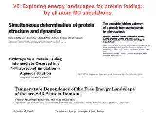
1. V5: Exploring energy landscapes for protein folding:by all-atom MD simulations Optimization, Energy Landscapes, Protein Folding

2. The folded state How do you characterize the folded state of a protein? Optimization, Energy Landscapes, Protein Folding

3. Combining experiment with simulations Traditional procedures for the experimental determination of protein structures: X-ray crystallography + nuclear magnetic resonance (NMR) Both methods determine the average structure of a protein with high accuracy. However, the dynamical properties associated with backbone and side-chain mobilities are also crucial determinants of many aspects of protein behaviour, including stability, folding and function. Information about such dynamic processes can be obtained from a variety of different experimental techniques, most notably those detecting NMR relaxation phenomena. In addition, molecular dynamics simulations can provide insight into a wide variety of phenomena associated with molecular motion. The dynamical properties of proteins are, however, generally treated in isolation from the structure determination process, creating considerable uncertainty as to the distribution of conformations that is sampled by a protein under a given set of conditions. Lindorff-Larsen et al. Nature, 433, 128 (2005) Optimization, Energy Landscapes, Protein Folding

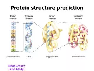
4. Cross-validation of ubiquitin structures Here: describe a method of determining protein structures in which information about the average structure is combined with explicit information obtained from NMR relaxation experiments about the structural variability in solution. Method is called „dynamic ensemble refinement (DER)“ Its performance is illustrated on human ubiquitin, for which a comprehensive range of high-quality NMR data are available. We used experimentally determined order parameters (S2) for the native state of ubiquitin as well as distance information from nuclear Overhauser effect (NOE) data as restraints in molecular dynamics simulations. The order parameters contain atomic-detailed information about the amplitude of molecular motion on a picosecond to nanosecond timescale, and thus about the variability of the native state ensemble on this timescale. By requiring that a set of ubiquitin conformations is simultaneously consistent with both the NOE data and the S2 restraints we obtain an experimental ensemble that represents both the structure and the dynamical variability in the native state of ubiquitin. Lindorff-Larsen et al. Nature, 433, 128 (2005) Optimization, Energy Landscapes, Protein Folding

5. Cross-validation of ubiquitin structures Structure determination was performed by solvating ubiquitin in a shell of 595 TIP3P water molecules and carrying out eight cycles of simulated annealing using an energy function of the form: Etot = ECHARMM +ENOE + ES2 : In this expression, ECHARMM is the CHARMM22 force-field energy and ENOE and ES2 are the energies due to the NOE and S2 restraints, respectively. NOE-derived distance restraints and experimental S2 values were obtained from the literature. As the experimental NOEs and S2 values are averages over a large ensemble of molecules, we enforced these restraints on an average calculated over a computer-generated ensemble. The restraints were applied using biased molecular dynamics in combination with ensemble simulations as described. The X-ray rapper ensemble was determined as described previously. A 6-ns unrestrained molecular dynamics simulation was performed essentially as described previously. Lindorff-Larsen et al. Nature, 433, 128 (2005) Optimization, Energy Landscapes, Protein Folding

6. Determination of ensembles of structures We used biased molecular dynamics (BMD) in combination with ensemble simulations of ubiquitin to obtain structural ensembles that satisfy simultaneously both sets of restraints. The simulation of a set of 16 copies, or replicas, of the protein provides results that are well converged in simulations using S2 values as restraints. In BMD the restraint energy is implemented as: In this expression, Nrepis the number of replicas, X corresponds to either NOE or S2, Xis a force constant associated with the restraint and 0(t) is defined as: Lindorff-Larsen et al. Nature, 433, 128 (2005) Optimization, Energy Landscapes, Protein Folding

7. Determination of ensembles of structures In the case of NOE restraints: in which we allow dcalcij to vary freely between its experimental upper and lower bounds, NNOEis the number of NOEs and the calculated distances derived from these correspond to r-3 weighted averages calculated over the ensemble of molecules: For S2 restraints: in which NS2 is the number of S2-restraints . 112 experimental S2 values taken from the literature after excluding values associated with large experimental uncertainties. NOE derived distance restraints were obtained from the PDB. Lindorff-Larsen et al. Nature, 433, 128 (2005) Optimization, Energy Landscapes, Protein Folding

8. Cross-validation of ubiquitin structures Cross-validation of ubiquitin structures by comparison with independently determined NMR data. Calculation of residual dipolar couplings (RDCs) (a) and sidechain scalar couplings (b). The NMR data were back-calculated from an ensemble of conformations that was determined using DER. The data point labels in a describe the atoms between which the RDCs were measured. In b, 3J NC and 3J CC are scalar couplings between the side-chaing carbon and the backbone amide nitrogen and carbonyl carbon, respectively. Lindorff-Larsen et al. Nature, 433, 128 (2005) Optimization, Energy Landscapes, Protein Folding

9. Variability in structural ensembles of ubiquitin a, Backbone trace of 15 representative conformations obtained from a clustering procedure. The structures are coloured from the N terminus (red) to the C terminus (blue) and are traced within an atomic density map representing the 20% amplitude isosurface of the density of atoms in the polypeptide main chain. The RMSD values of backbone (C) atoms (b) and side-chain atoms (c) in ubiquitin ensembles were determined by dynamic-ensemble refinement, NMR, X-ray diffraction and molecular dynamics (MD) simulations. Lindorff-Larsen et al. Nature, 433, 128 (2005) Optimization, Energy Landscapes, Protein Folding

10. Liquid-like mobility of side chains in the DER ensemble a, Joint distribution of the 1 dihedral angles in Ile 13 and Leu 15 in our 128 conformer ensemble (black), the crystal structure (red), the X-ray rapper ensemble (orange) and the published NMR ensemble (green). b, Four structures chosen from our DER ensemble to represent the four groupings of dihedrals evident in a; the four structures are arranged to match the four regions. Heavy atoms in the side chains of Ile 13 and Leu 15 are shown as van der Waals spheres (Ile 13 is located to the right of Leu 15). Lindorff-Larsen et al. Nature, 433, 128 (2005) Optimization, Energy Landscapes, Protein Folding

11. Variability in structural ensembles of ubiquitin c, Distribution of side-chain 1 and 2 dihedral angles of selected hydrophobic residues. Colouring scheme as in a. In some of the plots the histograms of dihedral angles for the X-ray, NMR and rapper structures overlap. Lindorff-Larsen et al. Nature, 433, 128 (2005) Optimization, Energy Landscapes, Protein Folding

12. Variability in structural ensembles of ubiquitin Quantifying backbone and side-chain variability in ubiquitin ensembles by comparison of experimental and back-calculated order parameters. In addition, the q-factors for a set of backbone RDCs are given for the individual ensembles. a, 128 conformer DER ensemble from this work using both NOEs and S2 values as restraints (q = 26%). b, X-ray rapper ensemble (q = 24%). c, The published NMR ensemble (q = 14%). d, 64 conformer ensemble from this work using NOEs enforced as restraints on a single conformer (q = 23%). e, 128 conformer ensemble from this work using NOEs enforced as restraints on an ensemble of molecules (q = 24%). f, Ensemble obtained from MD simulations (q = 52%). low values for q mean good agreement with experiment. Compare to R-Factor in crystallography. Lindorff-Larsen et al. Nature, 433, 128 (2005) Optimization, Energy Landscapes, Protein Folding

13. Significance for understanding protein behavior Shown here: combination of experimental parameters with MD simulations extends conventional structure determination methods to include accurate atomistic description of the conformational variability of the native states of proteins. Applying DER to ubiquitin shows that the native state must be considered as a heterogenous ensemble of conformations that interconvert on the ps to ns timescale, as well as populating more expanded conformations arising from rare but large fluctuations on much longer timescales, such as those revealed by H-exchange experiments. Many side chains, even in the core of the protein, occupy multiple rotameric states and can be considered to have liquid-like characteristics. Lindorff-Larsen et al. Nature, 433, 128 (2005) Optimization, Energy Landscapes, Protein Folding

14. Simulating the folding process How long does protein folding take? What timescale can we bridge by MD simulations?  Can we simulate a folding process? Optimization, Energy Landscapes, Protein Folding

15. Folding simulations Can one simulate a folding process by MD simulations? 1998 1 s simulation of 36-residue villin headpiece exp. folding time: between 10 – 100 s, Tm = 70 C - contains 3 short helices (NMR) connected by loop and turn - closely packed hydrophobic core 4 months of CPU time on 256 processor Cray T3D and T3E Optimization, Energy Landscapes, Protein Folding

16. Folding of villin headpiece unfolded partially folded native structures comparison of native (red) most stable cluster and most stable cluster (blue) Duan & Kollman, Science 282, 740 (1998) Optimization, Energy Landscapes, Protein Folding

17. Folding of villin head piece (A) fractional helical content (C) Radius of gyration and RMSD from native (B) fractional native content (D) solvation free energy (Eisenberg params) Duan & Kollman, Science 282, 740 (1998) Optimization, Energy Landscapes, Protein Folding

18. Folding of villin headpiece Pathways of folding events. Most populated clusters (circles) and transitions between them. Simulation able to probe early folding events . Burst phase (hydrophobic collapse) appears reasonable. Duan & Kollman, Science 282, 740 (1998) Optimization, Energy Landscapes, Protein Folding

19. Simulating the folding process Can we simulate the folding free energy landscape more efficiently + more exhaustively?  Combine MD with experiment. Optimization, Energy Landscapes, Protein Folding

20. All-atom MD simulations to study protein folding What do we want to learn? (1) Structure prediction starting from unfolded state? Currently too time consuming (sampling insufficient) May not work at all (force fields currently inadequate  don‘t stabilize folded state (F) over unfolded states (U) or intermediates (I) (2) „Ab initio“ characterization of folding pathway Difficult, but may work (3) Influence of external conditions (T, p) on folding pathway Well suited (4) Characterization of unfolded state and of transition state ensemble Optimization, Energy Landscapes, Protein Folding

21. All-atom MD simulations to study protein folding „The complete folding pathway of a protein from nanoseconds to microseconds“ Mayor, ..., Valerie Daggett, Alan R. Fersht, Nature, 421, 863 (2003) Combination of experiment - site directed mutagenesis - -value analysis - Trp fluorescence - NMR and molecular dynamics unfolding simulations Engrailed homeodomain: 61-residue -helical protein - fastest unfolding and one of the fastest folding proteins Optimization, Energy Landscapes, Protein Folding

22. Folding behavior Protein collapses within a microsecond to give an intermediate which much native -helical secondary structure. This is the major component of the denatured state under folding conditions. In general, F is typically more stable than U by only 5 – 15 kcal/mol. For En-HD, free energy difference only 2.5 kcal/mol. Introduce Ala  Leu mutant at position 16 (L16A): deletes stabilizing tertiary interactions without introducing a side chain that is likely to make new specific interactions Ala  Leu mutants often destabilize proteins by 4 – 5 kcal/mol. Also here, L16A-En-HD is unfolded Optimization, Energy Landscapes, Protein Folding

23. Characterization of En-HD and a L16A mutant a, Aromatic region of the 1H-NMR spectra of WT and L16A. Dispersion of the aromatic chemical shifts was lost in L16A (25 °C). b, Far-ultraviolet CD spectra of WT (25 and 95 °C) and L16A (25 °C). c, 15N-{1H} heteronuclear NOE data of WT (grey bars) and L16A (black circles) at 25 °C. The low NOE values for L16A indicate its higher flexibility. d, Deviations in chemical shift from reported random coil values in p.p.m. of WT (grey bars) and L16A (black circles) at 25 °C. No detectable native tertiary interactions, but contains most of its -helical structure backbone is very dynamic contains most of its -helical structure Optimization, Energy Landscapes, Protein Folding

24. Interpretation of experiments The denatured state revealed by L16A had the characteristic of a folding intermediate with much of the correct native secondary structure. X-ray scattering in solution  radius of gyration increased by 33% Optimization, Energy Landscapes, Protein Folding

25. Helices are more stable than entire protein Protection factors for the amide groups of wild-type En-HD, calculated from the 1H/2 H-exchange experiments at 5 °C. A value of 1 is given to those residues for which protection was not observed. The expected protection factor from a two-state fit of the denaturation curves is the thick grey line. En-HD in 2H2O : 2.8 kcal/mol thermal stability. Free energy of opening amide groups in helices: 3.4 kcal/mol.  The completely open denatured state of En-HD is ca. 1 kcal mol less stable than the dominant denatured state with considerable native -helical content. Optimization, Energy Landscapes, Protein Folding

26. Representative structures from MD simulations Generate folding intermediates by thermal denaturation simulations which are the quenched (cooled) to 25° C. a , Snapshots for the transition-state (TS) ensembles identified from wild-type (WT) simulations at different temperatures (61 ns at 75 °C, 1.985 ns at 100 °C and 0.26 ns at 225 °C), the intermediate (I) state (10-ns snapshots from the wild-type and L16A 225 °C trajectories quenched to 25 °C) and the unfolded (U) state (represented by the 40-ns WT 225 °C structure). The native helical segments are coloured as follows: red, residues 10–22; green, residues 28–38; blue, residues 42–55. Aromatic side chains are shown in magenta. b , Structures from the wild-type 225 °C denaturation simulation shown in reverse, to illustrate a probable folding pathway of the protein to reach the native (N) state. Simulated folding intermediates have extensive content of secondary structure. Optimization, Energy Landscapes, Protein Folding

27. Rate constants for folding and unfolding Monitor fluorescence of the single Trp residue after a laser-induced temperature jump of the sample.  experimental measurement of folding/unfolding rate constants Optimization, Energy Landscapes, Protein Folding

28. Kinetics of folding and unfolding a, Laser-heating T-jump of En-HD to 25 °C; data after 800 ns fitted to a double exponential. c, The L16A mutant of En-HD, T-jumped to 25 °C (Joule heating), showed only the fast phase. d, Observed relaxation rate constants (k) versus T. Solid curves were derived from combining k with equilibrium data from calorimetry. The filled red circles are results from NMR line-broadening analysis. Optimization, Energy Landscapes, Protein Folding

29. Structure of the transition state between N and I Analyze TS structure by  value analysis: -Werte measure the folding rate of a mutant k relative to wild-type and the change of the protein stability G0.  values are a measure of the degree of native structure in the transition state; 0 implies denatured, 1 implies fully native. Experimental data for 16 mutations.  values computed from the MD ensembles correlate very well (0.86) with experiment. Optimization, Energy Landscapes, Protein Folding

30. Complete folding pathway of En-HD by exp and simulation U is the quenched 40-ns snapshot from the simulation at 225 °C; I is the denatured state under 'physiological conditions'. The 10-ns structure from the high-T MD simulation is enclosed in the grey molecular envelope obtained by X-ray scattering. TS is the transition state between I and N, the native state. The simulated structure is from the transition state ensemble for the wild-type at 100 °C (1.985 ns). Structures are positioned according to their relative solvent accessibilities (T ), as obtained from the dependence of the rate constants on urea concentration. - Good agreement between exp and simulation. - Intermediate is on the pathway. Protein does not fold by an intermediate that must unfold to be productive. Optimization, Energy Landscapes, Protein Folding

31. Optimization, Energy Landscapes, Protein Folding

32. Folded structure The src-SH3 domain is a 56-residue -barrel protein. - two hydrophobic sheets orthogonally packed to form the hydrophobic core of the protein. src-SH3 has been shown to fold rapidly in a two-state manner. Optimization, Energy Landscapes, Protein Folding

33. Folded structure The transition state, characterized through -value analysis, was found to be unusually polarized, with the first sheet (2-3-4) of the hydrophobic core mostly formed while the rest of the protein remained unstructured. The term polarized reflects the fact the transition state is not diffuse in nature, but rather shows structure in only a specific portion of the protein (here, the first hydrophobic sheet). Homologous SH3 domains showed very similar transition states, intimating that the folding of this motif is governed by topological rather than energetic factors. Guo, Lampoudi, Shea Proteins, 55, 395 (2004) Optimization, Energy Landscapes, Protein Folding

34. Folded structure Earlier work focused on investigating the folding behavior of this protein under very native conditions, as well as near the folding transition temperature Tf. Folding was observed to be downhill at room temperature, with no significant barriers appearing in the free energy projected onto an order parameter , related to the number of native contacts. At 343 K (near the folding transition temperature), on the other hand, two barriers were present in the free energy plots. The major barrier, corresponding to the transition state barrier, occurred early in the folding process, while the smaller one, appearing in the later stages of folding, was identified as a desolvation barrier for folding. Optimization, Energy Landscapes, Protein Folding

35. Simulation Details PDB code 1SRL CHARMM package, CHARMM force field, TIP3P bond lengths constrained by SHAKE, t = 2 fs, Verlet Leap-frog integrater, particle mesh Ewald method. generation of folding trajectories from the unfolded state to the native state would be prohibitively costly. Rather, we generate free energy surfaces in a computationally, tractable manner by using extensive importance sampling MD simulations. Step 1: characterize the native state of the protein through 2 2-ns MD simulations at 298 K. Two descriptors of the native state, the number of native contacts, and the number of hydrogen bonds are defined from the native-state simulations. Native contact between two nonadjacent residues is formed if the center of geometry of their side-chains is within 6.5 Å. A hydrogen bond is formed if the distance between the backbone hydrogen and oxygen of two residues is less than 2.5 Å.  57 native contacts and 19 native hydrogen bonds. Optimization, Energy Landscapes, Protein Folding

36. Simulation Details Step 2: perform three 2-ns high-temperature unfolding simulations (400–450 K) to generate an ensemble of structures spanning the unfolded to the folded state. Cluster structures by hierarchical clustering scheme, using the number of native contacts, the number of native hydrogen bonds, and the protein solvation energy in the dissimilarity function.  76 cluster centers. These clusters centers are then used as the “initial conditions structures” for the biased sampling at the four temperatures considered: 298 K, 323 K, 343 K, and 363 K. Step 3: resolve each of the cluster centers, followed by 100–200 ps of NPT equilibration at the relevant temperature. Biased sampling, using a harmonic restraint in the fraction of native contacts () was then performed on each cluster center. The biased sampling was performed for 400–800 ps per structure, using a force constant between 500 and 1000 Kcal/mol. All production runs were performed at constant volume. Final step: combine sampling data using a constant temperature Weighted Histogram Analysis Method (WHAM). The density of states was then used to generate free energy surfaces at different temperatures as a function of the descriptors. Optimization, Energy Landscapes, Protein Folding

37. Definition of order parameter A number of parameters were used as folding metrics, including the backbone radius of gyration, the number of native contacts, the number of native hydrogen bonds (Nhb), and the number of core water molecules (Nwat). Water molecules residing inside an 8 Å sphere centered on geometrical center of the protein core were counted as core water molecules. We also used the fraction of native contacts () in the biased umbrella sampling, following the work of Brooks and coworkers. First the state of each contact x(i) is set to 1 if the distance d(i) between the centers of geometry of the side-chains is less than the cutoff K (6.5 Å), and to 0 if the distance is larger than the cutoff plus a given tolerance (“tol”, 0.3 Å) using the continuous function The fraction of native contacts is the sum of x(i) over all contacts. It is separated into Nbins (19) bins of width y (0.0526), with  = 1 and 0 representing the completely folded and unfolded states, respectively. This definition is advantageous over the number of native contacts, as it provides a continuous order parameter. The biased sampling along the order parameter is performed following the standard umbrella sampling protocol by adding a quadratic biasing potential of to the energy function. Optimization, Energy Landscapes, Protein Folding

38. Folded structure (a) pmf at 298 K as a function of . The free energy surface is downhill with a native basin at r 0.8. The stability of the native state is 3 kcal/mol. (b) pmf at 298 K as a function of  and radius of gyration, Rg (in Å). Contours are drawn every 1 kcal/mol. (c) pmf at 298 K as a function of  and the number of water molecules in the core. Contours are drawn every 0.6 kcal/mol. (d) Three high-temperature unfolding runs (T = 400 K) superimposed onto the free energy surface at 298 K. Folding at room temperature is down-hill! No significant barriers. Shea et al. PNAS 99, 16064 (2002) Optimization, Energy Landscapes, Protein Folding

39. Energy landscape at different temperatures Potential of mean force plotted as a function of  and radius of gyration Rg (in Å) at different temperatures. Contours are drawn every 1 kcal/mol. All curve L-shaped. 298K: downhill surface 323K: barrier at  = 0.8 343K: 2 barriers at  = 0.3 and at  = 0.8 363K: only 1 barrier at  = 0.3 323K 298K 343K 363K Guo, Lampoudi, Shea Proteins, 55, 395 (2004) Optimization, Energy Landscapes, Protein Folding

40. Formation of secondary structure Potential of mean force plotted as a function of  and number of native hydrogen bonds (Nhb) at different temperatures. Contours are drawn every 1 kcal/mol. PMFs are largely diagonal  HBs are formed concurrently with the native contacts. At all T, 5 HBs formed at  = 0.15 early collapse. At 343K, U is more stable than F. Higher barriers 298K 323K 343K 363K Guo, Lampoudi, Shea Proteins, 55, 395 (2004) Optimization, Energy Landscapes, Protein Folding

41. Nature of folding barriers Probability of native contact formation map of the structures residing at the top of the transition state ( = 0.3) barrier at (a) 343 K (upper quadrant) and 363 K (lower quadrant), and (b ) 298 K (upper quadrant) and 323 K (lower quadrant). The barrier has not shifted with temperature, and the structures at both temperatures are very similar in nature. Contacts are formed in the first hydrophobic sheet of the protein, while the remainder of the protein remains unstructured. Guo, Lampoudi, Shea Proteins, 55, 395 (2004) Optimization, Energy Landscapes, Protein Folding

42. Probabilities of hydrogen bonds Probabilities of hydrogen bond (PHB) before (  = 0.7) and after (  = 0.9) the second barrier at 323 K. Prior to the barrier most hydrogen bonds in 2- 3- 4 have high probabilities except in the loop regions, but those inside 5- 1- 2 and between sheets have intermediate PHB; after the barrier, all hydrogen bonds have high PHB. Guo, Lampoudi, Shea Proteins, 55, 395 (2004) Optimization, Energy Landscapes, Protein Folding

43. Solvation of hydrophobic core Potential of mean force plotted as a function of  and number of water molecules inside the core (Nwat) at different temperatures: (a) 298 K; (b) 323 K; (c) 343 K; (d) 363 K. Contours are drawn every 1 kBT. Guo, Lampoudi, Shea Proteins, 55, 395 (2004) Optimization, Energy Landscapes, Protein Folding

44. Contact maps at T = 298 K (upper quadrant) and T = 343 K (lower quadrant) at (a) = 0.2 (pretransition state barrier), (b) = 0.4 (posttransition state barrier), (c) = 0.6 (predesolvation barrier), and (d) = 0.9 (native basin). Guo, Lampoudi, Shea Proteins, 55, 395 (2004) Optimization, Energy Landscapes, Protein Folding

45. Folding pathways Unfolding trajectories at 363 K are projected onto the -Rg-PMFs at different temperatures: (a) 298 K; (b) 323 K; (c) 343 K; (d) 363 K. Guo, Lampoudi, Shea Proteins, 55, 395 (2004) Optimization, Energy Landscapes, Protein Folding

46. Conclusions (SH3) High-temperature simulations High-T unfolding runs map qualitatively well onto low-T free energy surfaces. Evidence of multiple pathways for folding and unfolding. High-T simulations don‘t capture the desolvation barrier  important barriers at low-T may disappear at high temperatures leading to the loss of crucial information from such simulations. Optimization, Energy Landscapes, Protein Folding

47. Conclusions (SH3) Folding proceeds from unfolded state through an initial collapse of the protein involving the formation of its first hydrophobic sheet. This is followed by the formation of the second hydrophobic sheet, and finally by the packing of the two hydrophobic sheets. Folding near the transition temperature reveals 2 barriers: a major one at  = 0.3 that corresponds to the transition state barrier a smaller one at  = 0.8 corresponding to a desolvation barrier. Free energy surfaces below the folding transition temperature only show a significant desolvation barrier, surfaces above only exhibit a significant transition state barrier. Optimization, Energy Landscapes, Protein Folding