Download

1 / 44
440 likes | 458 Views
This research focuses on improving the efficiency of stereo vision by selecting the most effective actions to disambiguate pixel matching. It explores the use of laser range finders and active stereo vision methods. The study includes experimental results and proposes a prototype solution.

E N D
Efficient Selection Of Disambiguating Actions for Stereo Vision Ronald Parr Duke University Joint work with Monika Schaeffer (Duke University)
These points match really well Traditional Stereo A benchmark stereo pair (Middlebury) How realistic is this? • Lots of texture • Small disparity range
????? What Robots See LSRC hallway Let’s go down this hallway without hitting a wall! • Huge disparity range • Large areas with little or no texture
Why not Use a Laser Range Finder? • Weight • Cost $$ • 2D or $$$ • (lack of) stealth • Power consumption • Low data bandwidth • Calibrated moving parts • Sensor can drive robot design
Alternatives • Sonar • 3D laser • Slow • $100K • Rotated/Rotating 2D laser • Retains nearly all disadvantages of 2D laser • Information per sweep: ~100 Kbits
Motivation Laser range finders Traditional Stereo Accurate Cheap Light Stealthy Benefits Expensive Bulky Impractical Calibrated mechanics Fails where Robots need accuracy Problems
Motivation Active Stereo Vision (stereo + laser pointer) Accurate Cheap Light Stealthy Benefits Expensive Bulky Impractical Calibrated mechanics Fails where Robots need accuracy Problems
Active Stereo Vision • Take base stereo pair of images • Take stereo pair(s) with addition of laser line (only crude calibration needed) • Image subtraction isolates laser line • Line disambiguates pixel matchings between pair The laser line divides problem into two independent stereo problems.
Using the laser A real stereo pair of images Test set: Lain m x n x d: 600 x 900 x 160 An artificial stereo pair of images
Using the laser Shine laser Line in right image = line in ground Brighter in ground = farther right in left image Calculate laser lines using ground truth image
Using the laser These points match These segments match Extract laser lines and update matchings These points match These segments match Update matchings
But what about… • Bulk, size & cost? • Prototype is much larger than necessary • P/T head need not be high quality (calibration not needed) • Stealth & speed? • Only use laser when/where necessary • Plan laser aims to reduce entropy • This is our sensor planning problem
How is Stereo Different? • Extremely large event space • Millions of pixels/image • Hundreds of values for each pixels • Cost of inference is high • (naïve) one step lookahead is impossible • Our main result:Can determine aim point for the laser that maximizes expected entropy reduction (information gain) in same asymptotic complexity as one run of stereo
Doing Stereo • Bobick & Intille present stereo as a shortest path problem • Construct the Disparity Space Image (DSI) • Find the shortest path in linear time using dynamic programming • Path through DSI = Stereo Matching for a scanline • Costs: • Assume n pixels/scanline (thousands) • Max disparity level of d (hundreds) • O(nd) per scanline
Constructing the DSI The DSI takes on three equivalent forms: • A dxn image containing information about the quality of matchings for a scanline • An dxnx3 graphical structure where paths through the graph represent valid pixel matchings for the scanline • An n-state HMM with O(d) possible values per state.
Constructing the DSI As an image: • A pixel in the right scanline is a column in disparity space. • A pixel in the left scanline is a diagonal in disparity space. • The left and right values are run through a cost function to get the matching score.
Constructing the DSI As an image: • A pixel in the right scanline is a column in disparity space. • A pixel in the left scanline is a diagonal in disparity space. • The left and right values are run through a cost function to get the matching score. • Not shown: Occlusion penalties
M M M M R R R R L L L L M M M M d = j-1 R R R R L L L L cost: DL cost: s(i+1,j) M M M M d = j R R R R L L L L M M M M d = j+1 R R R R cost: DR L L L L x = i x = i+1 M M M M R R R R L L L L Constructing the DSI As a graph: • Each pixel in DSI image corresponds to three nodes representing the state of that pixel. • Transitions from pixel (i,j) • M, R, L to M of (i+1,j) • M, L to L of (i, j-1) • M, R to R of (i+1, j+1)
M M M M R R R R L L L L M M M M R R R R L L L L M M M M R R R R L L L L M M M M R R R R L L L L Si Si+1 M M M M R R R R L L L L Constructing the DSI As an HMM: • Ms and Rs within a column i are mutually exclusive, jointly exhaustive. Considered possible values to state Si • Ls in a column encode a more complicated set of transitions from Ms in the column to Ms in the next column
Finding the Shortest Path • DSI is a highly structured DAG • We define the set of predecessor nodes, Γ- • Graph traversed from bottom to top, left to right. • Shortest path can be found in linear time with dynamic programming. For node c,
Query Selection • To maximize expected benefits of laser aims, we need a distribution over outcomes • Arc costs considered unnormalized log probabilities • Forward/backward algorithm to calculate node probabilities. For node c: Calculated backwards. Γ+ is the successor set.
Query Selection • Stereo matching = Path through DSI • Path entropy through DSI measure of our confusion over the best path • Query strategy: Maximize expected reduction in entropy
Query Selection Use this observation from Anderson & Moore : For entropy H(x), path space P, and queries Qt: IG(Qt) = H(P) - H(P|Qt) symmetry of mutual information: IG(Qt) = H(Qt) - H(Qt|P) Markov property: IG(Qt) = H(Qt) - H(Qt|St) IG(Qt) = H(St) - H(St|Qt) Expected entropy after query Qt Linear time!
Updating the DSI • If the laser is detected in both images, we split the DSI into two independent sections. • Paths are funnelled through M node. left scanline right scanline There are no valid paths through these dead zones that match our observation. DSI
Updating the DSI • If the laser is detected in both images, we split the DSI into two independent sections. • Many subtle details (ask later…) Each side is now independent of the other.
Hinge Doorknob Copier Real World Implementation • Took roughly one base and 200 lasered 1000x650px images • Used all 200 images to establish “ground truth” • Recalled nearest laser aim to query to simulate real time aiming Original Right Image Our Ground Truth
Entropy Disparity map with no lasers entropy
Entropy After two laser aims
Entropy After nine laser aims
Results on existing images We also ran the algorithm on two sets of existing images, the Middlebury Benchmark set “cones”, and some artificially generated airport security camera style images with little texture. We used ground truth to generate fake laser lines. security cam cones
Conclusion • Computational properties • O(nd) complexity • No asymptotic penalty for planning laser actions • Practical benefits of hybrid system • Small • Inexpensive • Selective use of laser • Accuracy increases with laser use
Conclusion • Results • Shown to work on both fake and real world images • Far more accurate than stereo alone • Better than random or equally spaced aims Questions? Thanks to: Carlo Tomasi, NSF, SAIC, IAI, Sloan Foundation.
Updating the DSI • If the laser is detected in both images, we split the DSI into two independent sections. • Paths are funnelled through M node. Each side is now independent of the other.
Updating the DSI • The ordering constraint is an assumption that keeps the stereo algorithm linear. • It does not necessarily hold in the real world. • The laser sometimes picks up on this. left scanline right scanline DSI
Updating the DSI • The ordering constraint is an assumption that keeps the stereo algorithm linear. • It does not necessarily hold in the real world. • The laser sometimes picks up on this. left scanline right scanline Detectable because violations occur in previously established dead zones. DSI
Updating the DSI • The ordering constraint is an assumption that keeps the stereo algorithm linear. • It does not necessarily hold in the real world. • The laser sometimes picks up on this. left scanline right scanline Detectable because violations occur in previously established dead zones. DSI
Updating the DSI • Pixels in one image do not necessarily map one to one with pixels in the other image. • The borders of dead zones must be left possible, though improbable left scanline right scanline DSI
Query Selection • We could also calculate the expected path entropy reduction in linear time using dynamic programming... h(c) = p(c) + Σ(p(b)log(p(c))+h(b)) bє Γ-(c) Run forward to get the total path entropy, run in both directions to get path entropy though each node.