Static Electric Fields: Principles and Applications
Explore the spatial distribution and properties of electric fields, including electric potential, dipoles, flux density, capacitors, and more. Learn about Coulomb's law, Gauss's law, and the impact of electric fields on materials and devices.

Static Electric Fields: Principles and Applications
E N D
Presentation Transcript
Chapter 3. Static Electric Fields 3.1 Introduction • Field : Spatial distribution of a physical quantity, function of position • What we will learn in this year. - Static Electric Fields Electric field intensity, Electric potential, Electric dipole, Electric properties of materials, Electric flux density (Displacement Vector) Capacitors, Electrostatic Energy and Forces, Solutions of Electrostatic Problems - Static Electric Currents Ohm’s Law, Electromotive force, Kirchhoff’s Voltage and Current Law, Continuity equation, Power and Joule’s law, Resistance calculation - Static Magnetic Fields Magnetic flux density, Magnetic potential, Magnetic dipole, Magnetic properties of materials, Magnetic field intensity, Magnetic circuits, Inductors, Magnetostatic Energy and Forces and torques. - Time-varying Electromagnetic Fields (2nd Semester) Plane Waves, Reflection, Refraction, Transmission lines, Transients on Transmission lines, Smith Chart • Static Electric Fields - In electrostatics, electric charges (the sources) are at rest, electric field do not change with time, there is no magnetic fields. - Lightning, corona, St. Elmo’s fire, grain explosion - Oscilloscope, ink-jet printer, xerography, electret microphone, Digital Mirror Device
Electrostatics • Source charges are at rest (Test charges can move). • Electric fields do not change with time : no magnetic fields • Coulomb’s law • Basic law about the electric force between two charged bodies • Experimental law discovered by Charles de Coulomb in 1785. : Coulomb’s law F12 F21 Coulomb’s torsion balance
Electric field intensity : the force per unit charge that a very small stationary test charge experiences when it is placed in a region where an electric field exists. • Fundamental postulates of electrostatics in free space • Differential forms : • Integral forms : Here, q is a test (probe) charge, which means that it is small enough not to disturb the charge distribution of the source. If a charge q is placed in a region where an electric field E exists, it feels a force of F = qE volume charge density Divergence theorem Stokes’ theorem total charge enclosed in the surface S : Gauss’s law : Energy Conservation
Characteristics of electric fields (1) Charge (density) forms an electric field that diverges (for static and dynamic cases). (2) The electrostatic field is conservative (only for static case). Every point? : The total outward flux of the electric field intensity over any closed surface in free space is equal to the total charge enclosed in the surface divided by 0. Gauss’s Law This law is an expression of Kirchhoff’s voltage law in circuit theory. : The algebraic sum of voltage drops around any closed circuit is zero. (Line integral of electric field is voltage.) : The scalar line integral of the static electric field intensity around any closed path vanishes. Along C1 Along C2 Along C1 Along C2
Electric field due to a single point charge q (1) By Coulomb’s law The force felt by a small test charge q at P is By the definition of the electric field, (2) By Gauss’s law q
If the charge q is not located at the origin, but at the specific position whose position vector is represented as R´ , • Electric field due to multiple point charges : The principle of superposition applies here, and E is the vector sum of fields caused by all the individual charges. Example 3-1. 3.2 p78
Example 3-3 : Cathode-ray oscilloscope (electrostatic deflection) The electrostatic deflection system of a cathode-ray oscilloscope is depicted in Fig. 3-4. Electrons from a heated cathode are given an initial velocity by a positively charged anode (not shown). The electrons enter at z = 0 into a region of deflection plates where a uniform electric field is maintained over a width w. Ignoring gravitational effects, find the vertical deflection of the electrons on the fluorescent screen at z = L. Sol. * Inkjet printers are devices based on the principle of electrostatic deflection of a stream of charged particles.
Electric dipole • Electric dipole : two point charges of equal magnitude and opposite polarity +q and –q, separated by a small distance d (e.g. molecular scale polarization in dielectric materials) • Is an important entity in the study of electric field in dielectric media. • Determines the electrical and optical properties of the material. • Electric field due to an electric dipole Taylor expansion
(Cont’d) • Electric dipole moment p : the product of the charge q and the vector d : The electric field intensity of an electric dipole is inversely proportional to the cube of the distance R. It is the proof of the faster decrease of the electric field rather than a single charge.
Source coordinate! • Electric field due to a continuous distribution of charge • The electric field caused by a continuous distribution of charge can be obtained by integrating (superposing) the contribution of an element of charge over the charge distribution. A differential element of charge in dv΄ behaves like a point charge and its contribution to the electric field intensity at P is Therefore, the total electric field E at the point P due to a volume charge distribution (density)ρ is given by For the surface charge distribution, For the line charge distribution,
Example 3-4 : Electric field of an infinitely long, straight, line charge of a uniform density in air • By symmetry, cylindrical coordinate system (CCS) is adequate. • It is an accepted convention to use primed coordinates for source points • and unprimed coordinates for field points when there is a possibility of • confusion. The 2nd term (z-component) is an odd function of z, and thus vanishes (Please see the left figure). (For integration, let z = r tan )
Gauss's law and applications • Gauss's law : The total outward flux of the E-field over any closed surface in free space is equal to the total charge enclosed in the surface divided by 0. It provides a convenient method for determining the electric fields of charge distributions with some symmetry conditions. • How to use Gauss's law? (1) Check the given charge distributions are symmetric. (2) Choose the Gaussian surface S such that, from symmetry conditions, the magnitude of the electric field is constant and its direction is normal (or tangential) at every point of the surface S.
ds Er (top) Er (side) ds At the side surface : • Example 3-5 : Electric field of an infinite (uniform) line charge Sol. (Step 1) Check the symmetry :infinite symmetry. E field must be radial and perpendicular to the line charge ( ). (Step 2) Choose and draw the Gaussian surface. (Step 3) Evaluate the integral part of Gauss's law. At the top (bottom) surface : E ds no contribution (Step 4) Calculate the total charge Q enclosed by the surface. (Step 5) Determine E by equating both sides of Gauss's law.
Top surface : Bottom surface : • Example 3-6 : Electric field of an infinite (uniform) planar charge Sol. (Step 1) Check the symmetry :infinite symmetry. E field must be normal to the sheet of charge ( ). ( (Step 2) Choose and draw the Gaussian surface. (Step 3) Evaluate the integral part of Gauss's law. (Step 4) Calculate the total charge Q enclosed by the surface . (Step 5) Determine E by equating both sides of Gauss's law.
Outside the charge cloud, the E field is exactly the same asthough the total charge is concentrated on a single point charge at the center. • This is true, in general, for a spherically charged region even though is a function of R. • special property of the spherical charge distribution. • Example 3-7 : Electric field of a spherical cloud of electrons (volume charges) Sol. Spherical symmetry condition Draw spherical Gaussian surface.
Electric potential • Concept of electric potential • In electric circuits, we work with voltages and currents, not electric or magnetic fields. • Electric potential is the same as voltage : The voltage V between the two points in the circuit represents the amount of work, or potential energy, required to move a unit charge between the two points. • Electric potential as a function of electric field • If we attempt to move the charge along the positive y-direction, we will need to provide an external force Fext to counteract Fe, which requires the expenditure of energy. • The work done in moving any object by is • The differential electric potential energy dW per unit charge is called the differential electric potential (or differential voltage) dV.
The result of the line integral on the right-hand side of the above equation should be independent of the specific integration path taken between points P1 and P2 • (See lecture note 4-4) This requirement is mandated by the law of conservation of energy. • In electric circuits, the voltage at a point in a circuit is • the voltage difference with respect to a conveniently chosen • point at which a reference voltage of zero is assigned (ground). • The reference potential point is usually chosen to be at infinity. reference point of V = 0 (infinity) • Potential difference • Potential difference : amount of work done against the electric field to move a unit charge from one point to another point The potential difference between any two points is obtained by integrating differential electric potential along any path between them. In electrostatics, the potential difference between two points is uniquely defined. • Electric potential (or voltage) at a point in space
Equipotential surface Force lines (flux lines) • Electric field from the electric potential In lecture 5-5, we noticed that . Also, from eq. (2-88), . By equating these two equations, we conclude that (1) The inclusion of the negative sign is necessary in order to conform with the convention that in going against the E field the electric potential V increases. (2) When we defined the gradient of a scalar field, the direction of (i.e. E) is normal to the surfaces of constant V : field lines are everywhere perpendicular to equipotential lines and equipotential surfaces.
Equipotential lines • Electric potential due to point charges • For a single point charge q at the origin, • The potential difference between any two points • The potential difference is determined by only two endpoints. • No work is done from P1 to P3. • Electric potential due to the multiple point charges
[HW] See Example 3-8. Since d << R, the lines R1 and R2 are approximately parallel to each other. Hence, Electric field can be obtained by taking negative gradient of the potential V. (d << R) Electric potential of an electric dipole
For the single point charge, For the volume charge distribution, For the surface charge distribution, For the line charge distribution, • Electric potential due to a charge distribution • The approach is the same as the cases of electric field equations. • The electric potential due to a continuous charge distribution confined in a given region is obtained by integrating the contribution of an element of charge over the charged region.
[HW] Solve Example 3-10. • For very large z, When the point of observation is very far away from the charged disk (far field), The E field approximately follows the inverse square law as if the total charge were concentrated at a point. Example 3-9 : Electric field on the axis of a circular disk carrying a surface charge density
Electrical properties of materials • Electromagnetic constitutive parameters of a material medium • Electrical permittivity, • Magnetic permeability, • Conductivity, : a measure of how easily electrons can travel through the material under the influence of an external electric field. • A material is said to be : • homogeneous : if its constitutive parameters do not vary from point to point • isotropic : if its constitutive parameters are independent of direction • Classification of materials based on their electrical property • Conductors (metals) : having a large number of loosely attached electrons in the outermost shells of the atoms migrating easily with or without an electric field • Dielectrics (insulators) : having electrons tightly held to the atoms difficult to detach them even under the influence of an electric field • Semiconductors : their conductivities fall between those of conductors and insulators
Band Theory (a) Probability density function of an isolated hydrogen atom (b) Overlapping probability density functions of two adjacent hydrogen atoms (c) The splitting of the n = 1 state. As atoms are brought together from infinity, the atomic orbits overlap and give rise to bands. Outer orbits overlap first. The 3s orbits give rise to the 3s band, 2p orbits to the 2p band, and so on.
The splitting of the 3s and 3p states of silicon into the allowed and forbidden energy bands. Schematic of an isolated silicon atom. electron Insulator Conduction band hole Valence band Semiconductor Hole: bubble in water, unoccupied chair in crowded theater unoccupied state in valence band
Conductors • Conductors : materials having a lot of free electrons, resulting in high conductivities • Most metals : ~ 106 to 107 S/m (c.f. good insulators : ~ 10-10 to 10-17 S/m) • Perfect conductor : = (c.f. perfect dielectric : = 0) • Superconductor : having a practically infinite conductivity and Meissner effectat very low temperature (Meissner effect: the effect of expelling magnetic field ) • Ohm's law for conductors The drift velocity ue of electrons in a conducting material is given by The current density in a conducting medium containing a volume charge density e (electrons) moving with a velocity u is . Therefore, • In a perfect dielectric ( = 0) : J = 0 regardless of E (However, there is no perfect dielectrics.) • In a perfect conductor ( = ) : E = J/ = 0 regardless of J (However, there is no perfect conductor, but superconductor.) (e : electron mobility) : point form of Ohm's law (for conductors)
Example: Resistance and speed of electrons in conductor. Find the resistance of a 1 mile (1.609 km) length of #16 copper wire, which has of 1.291 mm. This #16 wire can safely carry about 10 Adc. Speed of electron? Very slow!!!
Properties of conductors (1) Inside a (perfect) conductor (under static conditions): Inside a conductor, no volume charge density can exist. All charges move to the surface of a conductor and redistribute themselves in such a way that both the charge densities and the electric field inside vanish. (2) Under static condition, the electric field E on the conductor surface is everywhere normal to the surface. Otherwise, the charges would move tangential to the surface. (3) A conductor under static condition is an equipotential medium Potential is constant inside a conductor and on the conductor surface. (4) Potential is continuous across any surfaces, but the electric field is not. The electric field may be discontinuous across the boundary that has a surface charge density.
Boundary condition at an interface between a conductor and free space (1) Normal component : Use Gauss's law. (2) Tangential component : Use . B. C. at a conductor/free space interface : • Uncharged conductor in an external static electric field Applied external field E0 moves electrons inside a conductor to the left, and the right end becomes charged positively. + + + + + - - - - - Induced field E1 E=0 Induced field E1 is formed inside the conductor and it makes the field inside the conductor zero. conductor External field E0
+ + + - - - - - + + - - - +Q + + + • Example 3-11 : A point charge surrounded by a spherical conducting shell (Ro, Ri). Find E and V everywhere. P1
Dielectrics in static electric field (1) • Polarization (分極) mechanism in dielectrics • The electrons in the outermost shells of a dielectric are strongly bound to the atom. • In the absence of an external electric field, the electrons in any material form a symmetrical cloud around the nucleus, with the center of the cloud being at the same location as the center of the nucleus. • When an external electric field is applied to dielectrics, it can polarize the atoms or molecules : distorting the center of the electron cloud and the location of nucleus. • The polarized atom or molecule may be represented by an electric dipole. Such induced dipoles set up a small electric field. This induced field (polarization field) modifies the electric field inside and outside of the dielectric material.
H+ H+ 105o O- • Dielectrics in static electric field (2) • Polarized medium • Within the dielectric material, the induced dipoles align themselves in a linear arrangement, into the direction of the applied external field. • Along the upper and lower edges of the material, the dipole arrangement exhibits a positive and a negative surface charge density, respectively. • If the polarization not uniform, a polariztionvolume charge density can be created inside the dielectric material. • Nonpolar and polar materials • Nonpolar material • Molecules do not have permanent dipole moments. • Polarized only when an external electric field is applied • Polar material • Molecular structure shows built-in permanent dipole moments in the absence of an external electric field (e.g. water)
Equivalent charge distributions of polarized dielectrics To analyze the macroscopic effect of induced dipoles, we define a polarization vector P. : P is the volume density of the induced dipole moments. (n is the number of molecules per unit volume.) The dipole moment dp of an elemental volume dv' is . This moment produces a potential : potential produced by polarized material of volume V'. A polarized dielectric can be replaced by an equivalent surface bound charge density (ps) and an equivalent volume bound charge density (p). divergence theorem
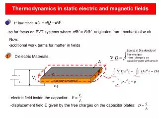
Electric flux density and dielectric constant Because a polarized material gives rise to an equivalent volume bound charge density p, the Gauss's law should be modified to include the effect of polarization. • Properties of medium • Linear, isotropic dielectrics : : Electric flux density(Electric displacement) * The use of the vector D enables us to write a divergence relation between the electric field and the distribution of free charges in any medium without the necessity of dealing explicitly with the polarization vector P or the polarization charge density p . * The D-field is medium-independent . Divergence theorem electric susceptibility absolute permittivity (permittivity) dielectric constant (relative permittivity) - Free space : 1.0 - Air : 1.00059
P P E E P E • Simple medium linear, homogeneous, isotropic medium nonlinear, homogeneous, isotropic medium Anisotropic medium Ferroelectric medium Tensor Biaxial medium Uniaxial medium
Example 3-12 : A point charge at the center of a spherical dielectric shell Dielectric problem : 1) find D instead of E, 2) find E, 3) find P from E.
+ + + + - + - - + - - + - - - (Cont'd) • Surface and volume bound charges (1) On the inner shell surface : (2) On the outer shell surface : (3) Inside the dielectric volume : Induced surface bound charges reduce the electric field in the dielectric made from the charge Q. • Dielectric strength • Dielectric breakdown : permanent damage under strong electric field • Dielectric strength : maximum E field that a dielectric material can withstand without breakdown (See Table 3-1) Field by Q + Field by polarization + + + +
Boundary conditions for electrostatic fields (1) Tangential component (2) Normal component Tangential component of an E field is continuous across an interface. Normal component of a D field is discontinuous across an interface where ‘free’ surface charge exists : the amount of discontinuity is equal to the free surface charge density. Where the reference unit normal is outward from 2. (p117) • If medium 2 is a conductor : (If medium 1 is free space, ) • Two dielectric are in contact with no free charges at the interface :
Example 3-14 : An interface between the dielectric sheet and free space A lucite sheet (r = 3.2) is introduced perpendicularly in a uniform electric field in free space. Determine Ei, Di, andPiinside the lucite. Sol) We assume that the introduction of the sheet does not disturb the original uniform electric field. (Why?) Only normal field components need to be considered. Where the reference unit normal is outward from 2. (p117) No free surface charge exists ! ② ①
rp εrr ro εrp • Example 3-16. Coaxial cable to carry electric power. The radius of inner conductor is determined by the load current, and the overall sized by the voltage and type of insulating material used. ri=0.4 cm, εrr(rubber)=3.2, εrp(polystyrene)=2.6. Design a cable that is to work at a voltage rating of 20 kV. In order to avoid breakdown due to voltage surges, the maximum electric field intensities in the insulating materials are not exceed 25% of their dielectric strength. ri a voltage rating of 20 kV
: CapacitanceC is the constant of proportionality. • Capacitance and capacitors • Capacitance of an isolated conductor Assume that a single conductor has charge Q and its potential is V. If we increase the charge to kQ, the potential is also increased to kV (Why?). The charge of a conductor and its potential is proportional to each other. • Capacitor : two conductors separated by free space or a dielectric medium • The capacitance of a capacitor depends on : • (1) Geometry of the capacitor (size, shape, relative • positions of two conductors) • (2) Permittivity of the medium between conductors
② ① (neglect fringing field.) +Q (1) Coordinate system : RCS (left figure) (2) Put charges +Q(upper) and –Q(lower) : The charges are assumed to be uniformly distributed over the conducting plate with surface charge density +s and –s. –Q • How to calculate the capacitance? (1) Choose an appropriate coordinate system (2) Assume charge +Q and –Q on the conductors (3) Find E from Q (4) Find V12 by evaluating the line integral of E from –Q to +Q (5) Find C by taking the ration Q/V12. • Example 3-17 : Capacitance of a parallel-plate capacitor
Important! Solve Example 3-19. • CS : CCS (left figure) • Put charges +Q(inner) and –Q(outer) • Find the E field by Gauss’s law. Assuming (Fringing field is also neglected.) Example 3-18 : Capacitance of a cylindrical capacitor
Series connection Parallel connection Series and parallel connections of capacitors
cii : coefficients of capacitance = ratio of charge Qi on and the potential Vi of the i-th conductor with all other conductors grounded. cij : coefficients of induction cii > 0, cij< 0 and cij = cji • Capacitances in multi-conductor systems • In the case of more than two conducting bodies in an isolated system,
V3 will not affect Q1, and vice versa : shielding Four conductor systems Electrostatic shielding (Faraday cage)
P3 q3 R23 R13 P2 R12 P1 q2 q1 • Electrostatic energy • Work needed to locate three point charges q1, q2, q3 at locations P1, P2, P3 Work needed to place a charge q at the point P is W = qV(P) . (1) Locating q1 at P1 : No work is needed because of no field. (2) Locating q2 at P2 : Work must be done against the E-field produced by q1. (3) Locating q3 at P3 : Work must be done against the E-field produced by q1 and q2. The total energy required to locate the three charges is
: electric potential at qk position caused by all the other charges • General expression for potential energy of a group of N discrete point charges • Two remarks (1) We can be negative. (2) We represents only the interaction energy (mutual energy) and does not include the work required to assemble the individual point charge themselves. • Units of energy : Joule (J) cf) electron-volt (eV) : work required to move an electron against a potential difference of 1 V 1 (eV) = 1.610-19 (J) • Electrostatic potential energy of a continuous charge distribution
= 0 for infinitely large volume, why? Electrostatic energy density, we: • Electrostatic energy in terms of field quantities V' : any volume including all the charges very large sphere with radius R. As we let R, (1) V and D fall off at least as fast as 1/ R and 1/ R2, respectively. (2) The area of the bounding surface S' increases as R2. The first surface integral term decreases as fast as 1/ R and will vanish as R.
b Rx V(Rx) • Three Methods to find electrostatic energy for assembling a uniform spherical volume charge densities of radius b.