Numerical Methods for Engineering MECN 3500
Numerical Methods for Engineering MECN 3500. Professor: Dr. Omar E. Meza Castillo omeza@bayamon.inter.edu http://www.bc.inter.edu/facultad/omeza Department of Mechanical Engineering Inter American University of Puerto Rico Bayamon Campus. Tentative Lectures Schedule. Finite Difference.

Numerical Methods for Engineering MECN 3500
E N D
Presentation Transcript
Numerical Methods for Engineering MECN 3500 Professor: Dr. Omar E. Meza Castillo omeza@bayamon.inter.edu http://www.bc.inter.edu/facultad/omeza Department of Mechanical Engineering Inter American University of Puerto Rico Bayamon Campus
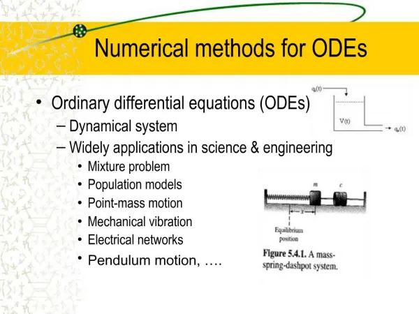
Finite Difference Best known numerical method of approximation
Course Objectives • To understand the theory of finite differences. • To apply FD to the solution of specific problems as a function of accuracy, condition matrix, and performance of iterative methods.
FINITE DIFFERENCE FORMULATION OF DIFFERENTIAL EQUATIONS finite difference form of the first derivative Taylor series expansionof the function f about the point x, The smaller the x, the smallerthe error, and thus the more accurate the approximation.
FINITE DIFFERENCE APPROXIMATION OF HIGHER DERIVATIVE • The forward Taylor series expansion for f(xi+2) in terms of f(xi) is • Combine equations:
Solve for f ''(xi): • This formula is called the second forward finite divided difference and the error of order O(h). • The second backward finite divided difference which has an error of order O(h) is
The second centered finite divided difference which has an error of order O(h2) is
High accurate estimates can be obtained by retaining more terms of the Taylor series. High-Accuracy Differentiation Formulas • The forward Taylor series expansion is: • From this, we can write
Substitute the second derivative approximation into the formula to yield: • By collecting terms: • Inclusion of the 2nd derivative term has improved the accuracy to O(h2). • This is the forward divided difference formula for the first derivative.
Example Estimate f '(1) for f(x) = ex + x using the centered formula of O(h4) with h = 0.25. Solution • From Tables
Error • Truncation Error: introduced in the solution by the approximation of the derivative • Local Error: from each term of the equation • Global Error: from the accumulation of local error • RoundoffError: introduced in the computation by the finite number of digits used by the computer
Introduction to Finite Difference • Numerical solutions can give answers at only discrete points in the domain, called grid points. • If the PDEs are totally replaced by a system of algebraic equations which can be solved for the values of the flow-field variables at the discrete points only, in this sense, the original PDEs have been discretized. Moreover, this method of discretization is called the method of finite differences. (i,j)
Discretization: PDE FDE • ExplicitMethods • Simple • No stable • ImplicitMethods • More complex • Stables ∆x ¬ ® y n+1 ∆y y n u m,n y n-1 x x x m-1 m m+1
Summary of nodal finite-difference relations for various configurations: Case 1: Interior Node
SolvingFiniteDifferenceEquations Heat Transfer Solved Problem
Error Definitions • Use absolute value. • Computations are repeated until stopping criterion is satisfied. • If the following Scarborough criterion is met Pre-specified % tolerance based on the knowledge of your solution
Using Excel Matrix Inversion Method =MMULT(A7:C9,E2:E4) =MINVERSE(A2:C4)
A large industrial furnace is supported on a long column of fireclay brick, which is 1 m by 1 m on a side. During steady-state operation is such that three surfaces of the column are maintained at 500 K while the remaining surface is exposed to 300 K. Using a grid of ∆x=∆y=0.25 m, determine the two-dimensional temperature distribution in the column. (2,3) (3,3) (1,3) (2,2) (3,2) (1,2) (2,1) (3,1) (1,1) Ts=300 K