PH0101 UNIT 2 LECTURE 2
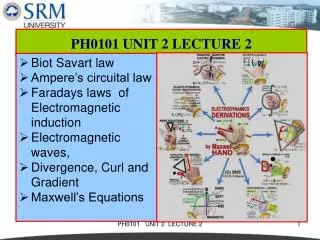
PH0101 UNIT 2 LECTURE 2. Biot Savart law Ampere’s circuital law Faradays laws of Electromagnetic induction Electromagnetic waves, Divergence, Curl and Gradient Maxwell’s Equations. Biot – Savart Law.

PH0101 UNIT 2 LECTURE 2
E N D
Presentation Transcript
PH0101 UNIT 2 LECTURE 2 • Biot Savart law • Ampere’s circuital law • Faradays laws of Electromagnetic induction • Electromagnetic waves, • Divergence, Curl and Gradient • Maxwell’s Equations PH0101 UNIT 2 LECTURE 2
Biot – Savart Law Biot - Savart law is used to calculate the magnetic field due to a current carrying conductor. According to this law, the magnitude of the magnetic field at any point P due to a small current element I.dl ( I = current through the element, dl = length of the element) is, In vector notation, PH0101 UNIT 2 LECTURE 2
Ampere’s circuital law • It states that the line integral of the magnetic field (vector B) around any closed path or circuit is equal to μ0 (permeability of free space) times the total current (I) flowing through the closed circuit. Mathematically, PH0101 UNIT 2 LECTURE 2
Faraday’s Law of electromagnetic induction • Michael Faraday found that whenever there is a change in magnetic flux linked with a circuit, an emf is induced resulting a flow of current in the circuit. • The magnitude of the induced emf is directly proportional to the rate of change of magnetic flux. • Lenz’s rule gives the direction of the induced emf which states that the induced current produced in a circuit always in such a direction that it opposes the change or the cause that produces it. d is the change magnetic flux linked with a circuit PH0101 UNIT 2 LECTURE 2
Electromagnetic waves • According to Maxwell’s modification of Ampere’s law, a changing electric field gives rise to a magnetic field. • It leads to the generation of electromagnetic disturbance comprising of time varying electric and magnetic fields. • These disturbances can be propagated through space even in the absence of any material medium. • These disturbances have the properties of a wave and are called electromagnetic waves. PH0101 UNIT 2 LECTURE 2
Representation of Electromagnetic waves PH0101 UNIT 2 LECTURE 2
Description of EM Wave • The variations of electric intensity and magnetic intensity are transverse in nature. • The variations of E and H are perpendicular to each other and also to the directions of wave propagation. • The wave patterns of E and H for a traveling electromagnetic wave obey Maxwell’s equations. • EM waves cover a wide range of frequencies and they travel with the same velocity as that of light i.e. 3 10 8 m s – 1. • The EM waves include radio frequency waves, microwaves, infrared waves, visible light, ultraviolet rays, X – rays and gamma rays. PH0101 UNIT 2 LECTURE 2
Divergence, Curl and Gradient Operations (i) Divergence • The divergence of a vector V written as div V represents the scalar quantity. div V = V = PH0101 UNIT 2 LECTURE 2
Example forDivergence PH0101 UNIT 2 LECTURE 2
Physical significance of divergence • Physically the divergence of a vector quantity represents the rate of change of the field strength in the direction of the field. • If the divergence of the vector field is positive at a point then something is diverging from a small volume surrounding with the point as a source. • If it negative, then something is converging into the small volume surrounding that point is acting as sink. • if the divergence at a point is zero then the rate at which something entering a small volume surrounding that point is equal to the rate at which it is leaving that volume. • The vector field whose divergence is zero is called solenoidal PH0101 UNIT 2 LECTURE 2
Curl of a Vector field Curl V= • Physically, the curl of a vector field represents the rate of change of the field strength in a direction at right angles to the field and is a measure of rotation of something in a small volume surrounding a particular point. • For streamline motions and conservative fields, the curl is zero while it is maximum near the whirlpools PH0101 UNIT 2 LECTURE 2
Representation of Curl (I) No rotation of the paddle wheel represents zero curl (II) Rotation of the paddle wheel showing the existence of curl (III) direction of curl • For vector fields whose curl is zero there is no rotation of the paddle wheel when it is placed in the field, Such fields are called irrotational PH0101 UNIT 2 LECTURE 2
Gradient Operator • The Gradient of a scalar function is a vector whose Cartesian components are, Then grad φ is given by, PH0101 UNIT 2 LECTURE 2
The magnitude of this vector gives the maximum rate of change of the scalar field and directed towards the maximum change occurs. • The electric field intensity at any point is given by, E = grad V = negative gradient of potential • The negative sign implies that the direction of E opposite to the direction in which V increases. PH0101 UNIT 2 LECTURE 2
Important Vector notations in electromagnetism div grad S = 1. 2. 3. 4. curl grad = 0 PH0101 UNIT 2 LECTURE 2
Theorems in vector fields Gauss Divergence Theorem • It relates the volume integral of the divergence of a vector V to the surface integral of the vector itself. • According to this theorem, if a closed S bounds a volume , then div V) d = V ds (or) PH0101 UNIT 2 LECTURE 2
Stoke’s Theorem • It relates the surface integral of the curl of a vector to the line integral of the vector itself. • According to this theorem, for a closed path C bounds a surface S, V dl (curl V) ds = PH0101 UNIT 2 LECTURE 2
Maxwell’s Equations Maxwell’s equations combine the fundamental laws of electricity and magnetism . The are profound importance in the analysis of most electromagnetic wave problems. These equations are the mathematical abstractions of certain experimentally observed facts and find their application to all sorts of problem in electromagnetism. Maxwell’s equations are derived from Ampere’s law, Faraday’s law and Gauss law. PH0101 UNIT 2 LECTURE 2
Maxwell’s Equations Summary PH0101 UNIT 2 LECTURE 2
Maxwell’s equation: Derivation Maxwell’s First Equation • If the charge is distributed over a volume V. Let be the volume density of the charge, then the charge q is given by, q = PH0101 UNIT 2 LECTURE 2
The integral form of Gauss law is, (1) By using divergence theorem (2) From equations (1) and (2), (3) PH0101 UNIT 2 LECTURE 2
r Ñ · = E e 0 Electric displacement vector is (4) (4) (5) div div (5) (6) PH0101 UNIT 2 LECTURE 2
Eqn(5) × (or) div PH0101 UNIT 2 LECTURE 2
This is the differential form of Maxwell’s I Equation. (7) From Gauss law in integral form This is the integral form of Maxwell’s I Equation PH0101 UNIT 2 LECTURE 2
Maxwell’s Second Equation From Biot -Savart law of electromagnetism, the magnetic induction at any point due to a current element, dB = (1) In vector notation, = Therefore, the total induction (2) = This is Biot – Savart law. PH0101 UNIT 2 LECTURE 2
(3) replacing the current i by the current density J, the current per unit area is [ i =J . A and I . dl = J(A . dl) = J .dv] Taking divergence on both sides, (4) PH0101 UNIT 2 LECTURE 2
For constant current density (5) Differential form of Maxwell’s’ second equation By Gauss divergence theorem, (6) Integral form of Maxwell’s’ second equation. PH0101 UNIT 2 LECTURE 2
Maxwell’s Third Equation By Faradays’ law of electromagnetic induction, (1) By considering work done on a charge, moving through a distance dl. W = (2) PH0101 UNIT 2 LECTURE 2
The magnetic flux linked with closed area S due to the Induction B = If the work is done along a closed path, emf = (3) (4) PH0101 UNIT 2 LECTURE 2
(Integral form of Maxwell’s third equation) (5) = (6) PH0101 UNIT 2 LECTURE 2
(Using Stokes’ theorem ) = (7) Hence, (8) Maxwell’s’ third equation in differential form PH0101 UNIT 2 LECTURE 2
Maxwell’s Fourth Equation By Amperes’ circuital law, (1) We know, (or) B = μ0 H (2) Using (1) and (2) (3) (4) We knowi = PH0101 UNIT 2 LECTURE 2
Using (3) and (4) (5) We Know that We Know that (6) (6) (7) (7) (Maxwell’s fourth equation in integral form) PH0101 UNIT 2 LECTURE 2
Using Stokes theorem, (8) (8) (Using (7) and (8)) (Using (7) and (8)) (9) PH0101 UNIT 2 LECTURE 2
The above equation can also be written as (10) (11) Differential form of Maxwell fourth equation PH0101 UNIT 2 LECTURE 2
Have a nice day. PH0101 UNIT 2 LECTURE 2