Download
1 / 60
600 likes | 623 Views
This lecture provides an overview of wavefield imaging and inverse scattering techniques, including digital holographic microscopy, and discusses their applications, imaging performance, and experimental examples.

E N D
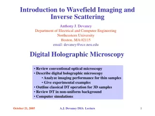
Introduction to Wavefield Imaging and Inverse Scattering Anthony J. Devaney Department of Electrical and Computer Engineering Northeastern University Boston, MA 02115 email: devaney@ece.neu.edu Digital Holographic Microscopy • Review conventional optical microscopy • Describe digital holographic microscopy • Analyze imaging performance for thin samples • Give experimental examples • Outline classical DT operation for 3D samples • Review DT in non-uniform background • Computer simulations A.J. Devaney IMA Lecture
Image Semi-transparent Object Condenser Objective Lens Optical Microscopy • Illuminating light spatially coherent over small scale: • Complicated non-linear relationship between sample and image • Poor image quality for 3D objects • Need to thin slice • Cannot image phase only objects: • Need to stain • Need to use special phase contrast methods • Require high quality optics • Images generated by analog process Remove all image forming optics and do it digitally A.J. Devaney IMA Lecture
I LO LI O Magnification and Resolution Pin hole Camera Magnification: M=LI/LO=I/O Real Camera I a δ δ=λ/2N.A. O a θ Resolution: N.A.=sin θ ≈ a/O O A.J. Devaney IMA Lecture
Fourier Analysis in 2D y Ky FT IFT ρ Kρ x Kx A.J. Devaney IMA Lecture
Propagating waves Evanescent waves Plane Waves k θ z γ A.J. Devaney IMA Lecture
Abbe’s Theory of Microscopy Lens focuses each plane wave at image point Plane waves Thin sample Image of sample Illuminating light Each diffracted plane wave component carries sample information at specific spatial frequency Diffracted light Max Kρ=k sin θ k θ z γ A.J. Devaney IMA Lecture
Basic Digital Microscope Plane waves Lens Illuminating light Image of sample Diffracted light Each diffracted plane wave component carries sample information at specific spatial frequency Plane waves Detector system Coherent light PC Image of sample Diffracted light Issues: Speckle noise, phase retrieval, numerical aperture A.J. Devaney IMA Lecture
Coherent Imaging Lens Image Thin sample Nature Analog Imaging Measurement plane Illuminating plane wave Computer Computational Imaging A.J. Devaney IMA Lecture
Coherent Computational Imaging Measurement plane Illuminating plane wave Computer Computational Imaging Propagation Undo Propagation Σ Σ0 Σ A.J. Devaney IMA Lecture
Plane Wave Expansion of the Solution to the Boundary Value Problem Σ ≡ z Σ0 A.J. Devaney IMA Lecture
Propagation in Fourier Space evanescent z propagating Propagation Σ z Σ0 propagating evanescent Σ Free space propagation (z> 0) corresponds to low pass filtering of the field data A.J. Devaney IMA Lecture
Undoing Propagation: Back propagation Propagation Backpropagation Σ Σ z z Σ0 Σ0 Σ Σ propagating evanescent Back propagation requires high pass filtering and is unstable (not well posed) A.J. Devaney IMA Lecture
Back propagation of Bandlimited Fields Propagation z Backpropagation Σ0 Σ Propagation Backpropagation A.J. Devaney IMA Lecture
Coherent Imaging Via Backpropagation Kirchoff approximation Backpropagation Plane wave Σ Σ0 • Very fast and efficient using FFT algorithm • Need to know amplitude and phase of field A.J. Devaney IMA Lecture
Limited Numerical Aperture Backpropagation a θ Σ0 z Σ PSF of microscope Abbe’s theory of the microscope A.J. Devaney IMA Lecture
Abbe Resolution Limit -k -k sin θ a θ Σ0 z k sin θ Σ k Maximum Nyquist resolution = 2π/BW=/2sinθ A.J. Devaney IMA Lecture
Phase Problem Gerchberg Saxon, Gerchberg Papoulis Multiple measurement plane versions Holographic approaches A.J. Devaney IMA Lecture
Camera # 2 Sample collimator Diffraction Plane # 1 Magnifying Lens Mirror Beam Splitter HE-NE Laser Sample collimator incident plane wave HE-NE Laser incident plane wave Beam Splitter Diffraction Plane # 2 Camera Camera # 1 The Phase Problem A.J. Devaney IMA Lecture
Beam splitter Spatial filter ¼ plate mirror Laser polarizer lens CCD mirror Beam splitter sample Digital Holographic Microscope 1024X1024 10 bits/pixel Pixel size=10 Mach-Zender configuration Two holograms acquired which yield complex field over CCD Backpropagate to obtain image of sample A.J. Devaney IMA Lecture
Retrieving the Complex Field ¼ plate Four measurements required A.J. Devaney IMA Lecture
Limited Numerical Aperture CCD sample Measurement plane a Sin θ=a/z<<1 θ z=44 m.m. a=6 m.m. N.A.=.13 Σ0 Fuzzy Images z Σ A.J. Devaney IMA Lecture
Pengyi and Capstone Team A.J. Devaney IMA Lecture
Scattered intensity Hologram 1 800 100 100 150 200 200 600 300 300 100 400 400 400 500 500 50 200 600 600 700 700 0 200 400 600 200 400 600 (a) (b) Hologram 2 700 100 600 200 500 300 400 400 300 500 200 600 100 700 200 400 600 (c) 5 μm Slit A.J. Devaney IMA Lecture
Reconstructed intensity image from CDH 600 500 50 400 100 300 150 200 200 100 100 200 300 400 500 600 (a) Reconstructed intensity image from PSDH 30 25 50 20 100 15 10 150 5 200 100 200 300 400 500 600 (b) Reconstruction of slit A.J. Devaney IMA Lecture
Hologram 1 Scattered intensity Hologram 2 Ronchi ruling (10 lines/mm) A.J. Devaney IMA Lecture
Reconstruction of Ronchi ruling A.J. Devaney IMA Lecture
Conventional Versus Backpropagated A.J. Devaney IMA Lecture
Phase grating A.J. Devaney IMA Lecture
Reconstruction of phase grating A.J. Devaney IMA Lecture
Salt-water specimen A.J. Devaney IMA Lecture
Reconstruction of salt-water specimen d m pixel size x=1.675 m A.J. Devaney IMA Lecture
Scattered intensity Hologram 1 600 800 50 50 500 600 400 100 100 300 400 150 150 200 200 200 200 100 250 250 0 50 100 150 200 250 50 100 150 200 250 (a) (b) Hologram 2 800 50 600 100 400 150 200 200 250 50 100 150 200 250 (c) Biological samples: mouse embryo A.J. Devaney IMA Lecture
Reconstruction of mouse embryo Intensity image by PSDH Phase image by PSDH 12 20 20 2 10 40 40 1.5 8 60 60 6 1 80 80 4 0.5 100 100 2 0 120 120 20 40 60 80 100 120 20 40 60 80 100 120 (a) (b) Conventional optical microscope 200 150 100 50 (c) A.J. Devaney IMA Lecture
Cheek cell A.J. Devaney IMA Lecture
Reconstruction of cheek cell A.J. Devaney IMA Lecture
Onion cell A.J. Devaney IMA Lecture
Thick Sample System ¼ plate Thick (3D) sample of gimbaled mount Many experiments performed with sample at various orientations relative to the optical axis of the system Paper with Jakob showed that only rotation needed to (approximately) generate planar slices Use cylindrically symmetric samples A.J. Devaney IMA Lecture
Thick Samples: Born Model Thick sample Σ Σ0 Born Approximation Determines 3D Fourier transform over an Ewald hemi-sphere A.J. Devaney IMA Lecture
Generalized Projection Slice Theorem Kρ Kz -kz The scattered field data for any given orientation of the sample relative to the optical axis yields 3D transform of sample over Ewald hemi-sphere A.J. Devaney IMA Lecture
Multiple Experiments Kρ Ewald hemi-spheres k Kz k Kρ √2 k Kz A.J. Devaney IMA Lecture
Born Inversion for Fixed Frequency Problem: How to generate inversion from Fourier data on spherical surfaces Inversion Algorithms: Fourier interpolation (classical X-ray crystallography) Filtered backpropagation (diffraction tomography) A.J.D. Opts Letts, 7, p.111 (1982) Filtering of data followed by backpropagation: FilteredBackpropagationAlgorithm A.J. Devaney IMA Lecture
Inverse Scattering Filtering followed by back propagation 3D semi-transparent object Computer Object Reconstruction Illuminating plane waves Essentially combine multiple 3D coherent images generated for each scattering experiment A.J. Devaney IMA Lecture
Inadequacy of Born Model ¼ plate Thick (3D) sample of gimbaled mount Addressed by DWBA model • Sample is placed in test tube with index matching fluid: Multiple scattering • Samples are often times many wavelengths thick: Born model saturates Adequately addressed by Rytov model A.J. Devaney IMA Lecture
Linearize Rytov Model Complex Phase Representation (Non-linear) Ricatti Equation A.J. Devaney IMA Lecture
Short Wavelength Limit Classical Tomographic Model A.J. Devaney IMA Lecture
Free Space Propagation of Rytov Phase propagation Within Rytov approximation phase of field satisfies linear PDE Rytov transformation A.J. Devaney IMA Lecture
Degradation of the Rytov Model with Propagation Distance Rytov and Born approximations become identical in far field (David Colton) Experiments and computer simulations have shown Rytov to be much superior to Born for large objects—Back propagate fieldthen use Rytov--Hybrid Model A.J. Devaney IMA Lecture
Rytov versus Hybrid Model N. Sponheim, I. Johansen, A.J. Devaney, Acoustical Imaging Vol. 18 ed. H. Lee and G. Wade, 1989 A.J. Devaney IMA Lecture
Potential Scattering Lippmann Schwinger Equation A.J. Devaney IMA Lecture
Mathematical Structure of Inverse Scattering Non-linear operator (Lippmann Schwinger equation) Object function Scattered field data Use physics to derive model and linearize mapping Linear operator (Born approximation) Form normal equations for least squares solution Wavefield Backpropagation Compute pseudo-inverse Filtered backpropagation algorithm Successful procedure require coupling of mathematics physics and signal processing A.J. Devaney IMA Lecture