Download
1 / 38
391 likes | 633 Views
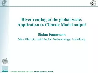
River routing at the global scale: Application to Climate Model output Stefan Hagemann Max Planck Institute for Meteorology, Hamburg. Closure of water balance between atmosphere and ocean in a coupled AO-GCM Impact of climate change on river flow

E N D
River routing at the global scale: Application to Climate Model output StefanHagemann Max Planck Institute for Meteorology, Hamburg
Closure of water balance between atmosphere and ocean in a coupled AO-GCM Impact of climate change on river flow Validation of the simulated hydrological cycle in climate models River routing required
Hydrological Cycle D. Gerten, PIK
Atmosphere MPI-ESM: Processes Sun Emissions Dynamics Aerosols Chemistry Land Surface Dust DMS CO2 MomentumEnergyWater Hydrology Photosynthesis Phenology Respiration Ocean Dynamics Sea-ice Biology Chemistry River runoff
Atmosphere ECHAM HAM MESSy/MOZART MPI-ESM: model components Sun Emissions Dust DMS CO2 JSBACH Land MomentumEnergyWater HD model PRISMcoupler MPI-OM HAMOCC Ocean
Concentrations (GHG, SO4) ECHAM5 T63L31 Sun MomentumEnergyWater ECHAM5 HD PRISMcoupler MPI-OM 1.5°L40 IPCC simulation:GCMmodel components
Lateral Soil Water Fluxes 1/2 º 1/6 º 1 d 1 h dx HD Model (Hydrological Discharge) Soil Hydrology Scheme Surface Runoff Overland Flow Hagemann & Dumenil (1998), Clim. Dyn. 14 Hagemann & Dumenil Gates (2001), J Geo. Res. 106 State of the art discharge model Applied and validated on global scale at 1/2 deg. Part of ECHAM5-MPIOM Time step: 1 day (internally 6 hours for riverflow) European version by Kotlarski: k = f (dx, innerslope, wetlands, lakes) Drainage Baseflow k = f (dx) Riverflow Gridbox Outflow Gridbox Inflow k = f (dx, dh/dx, wetlands, lakes)
Problems in HD model applications • 0.5 degree resolution is a good compromise beween the large-scale meteorological and the small-scale hydrological processes • Creation of realistic model orography is time consuming • Interpolation of climate model input required • Climate models often do not archive surface runoff and drainage separately • Land Surface Hydrology Model (LHSM) required
RCM Precipitation, Evaporation & 2m Temperature(daily values) Interpolation to 0.5 degree SimplifiedLand surface scheme Discharge HydrologicalDischarge model SL scheme/HD model LSHM as used in PRUDENCE Surface Runoff Drainage
Precipitation & 2m Temperature Snowpack Land Surface Single Soil Layer Drainage Runoff The SL Scheme Snow Rain Snowmelt Throughfall (Simplified Land surface scheme) Infiltration Evapotranspiration Time Step: 1 day Hagemann & Dümenil Gates, 2003
Precipitation & 2m Temperature Snowpack Land Surface Single Soil Layer Drainage Runoff The SL Scheme Evapotranspiration Snow Rain Snowmelt Throughfall (Simplified Land surface scheme) Infiltration Time Step: 1 day Hagemann & Dümenil Gates, 2003
Model validation and intercomparison Example: PRUDENCE 50 km x 50 km Current climate: 1961-1990 Future climate: A2 scenario 2071-2100 Hagemann & Jacob, Climatic Change,2007 Application to regional climate models
Baltic Sea catchment Elbe Rhine Danube
Discharge 1961-90 Large Spread
DischargeChanges 2071-2100
SL scheme forced by CRU2 data of precipitation and temperature for 1961-90 (Spin-up 1960). Daily variations are taken from ERA40 Application to observations and GCMs
A A A Baltic Sea A A A Danube Amur Mississippi Yangtze Kiang Nile Amazon Ganges/Brahmaputra Congo Parana Murray A = 6 largest Arctic Rivers = Mackenzie, N Dvina, Ob, Yenisey, Lena, Kolyma Large catchments are considered
Application to GCM: MPI-M IPCC simulations • Historical Climate (1860 – present), Focus: 1961-1990 • Scenarios (present to 2100), Focus: 2071-2100 • Low emission scenario: B1 • Moderate emission scenario: A1B • High emission scenario: A2 • GCM: ECHAM5 / MPI-OM • 3 ensemble members for historical control simulation and each scenario • Horizontal Resolution of ECHAM5: T63 ~ 200 km • Forcing with observed / prescribed (for scenarios) concentrations of CO2, Methane, N2O, CFCs, Ozone (Tropos-/Stratosphere), Sulfate Aerosols (direct and 1. indirect effect)
Summary • Problems in river routing • Interpolation from climate model grid to 0.5 grid required • Often a Land Surface Hydrology Model (LHSM) is required to force river routing model • Simulated discharge largely depends on the quality of precipitation and snowmelt used as forcing • Available discharge observations (e.g. from GRDC) often end in the 80s • Future Work • One aim of WATCH is to provide global LSHMs and methods to use forcing from climate models • These LSHMs shall include river routing, irrigation, dams, and groundwater schemes
© Canadian Space Agency, 1999 Thank you for your attention!
Summary of IPCC results • Trends for future climate (2071-2100 compared to 1961-90) • Pronounced changes of the hydrological cycle in all 3 scenarios, B1 changes tend to be smaller than for A1B and A2 whose changes are quite similar • Regional characteristics • High northern latitudes: Strongest warming in winter, generally enhanced hydrological cycle • Central Africa: Generally enhanced hydrological cycle • Pronounced drying in southern South Africa, southern Australia, and Mediterannean throughout the year • Drying in the dry seasons/Wetting in wet seasons for Danube (summer/winter), Indian and East Asian monsoon area (winter/summer), Amazon (summer-early fall/winter-spring)
Precipitation 1961-90 Common RCM problems