Download
1 / 39
420 likes | 474 Views
Explore the principles of finite state machines and sequential logic in embedded systems, including storage elements and shift register implementations. Learn about clock design considerations, timing, and testing methodologies for reliable circuit operation.

E N D
Embedded Systems Hardware: Storage Elements; Finite State Machines; Sequential Logic
fig_03_08 Finite state machine (FSM): High-level view Moore machine: output is a function of the present state only Mealy machine: output is a function of the present stare and the inputs fig_03_08
fig_03_09 Examples: Latch and register What is the difference? Shift register (shift right) fig_03_09 fig_03_10
fig_03_15 fig_03_15 fig_03_16 Verilog—shift registers; behavioral and structural (por=power on reset)
fig_03_18 fig_03_18 Parallel-in, serial-out shift register fig_03_19
fig_03_20 Linear feedback shift register (for providing random numbers, e.g.); Note: pullUp needed to prevent floating Reset pin on D flipflops fig_03_20, 3_21, 3_22
fig_03_23 “Dividers”: slow clock down, e.g. Simple divide-by-2 example fig_03_23,3_24
fig_03_25 Example: Asynchronous divide-by-4 counter [asynchronous 2-bit binary upcounter; ripple counter] Note: asynchronous because flip-flops are changed by different signals Note: if 1st stage output appears at time t0 + m, nth stage output appears at time t0 + nm; so this configuration is good for dividing the signal but using it as a ripple counter is prone to static and dynamic hazards Both outputs change: fig_03_25, 03_26, 03_27
fig_03_29 Synchronous dividers and counters (preferred): Example: 2-bit binary upcounter Inputs: DA = not A DB = A xor B fig_03_28, 03_29
Johnson counter (2-bit): shift register + feedback input; often used in embedded applications; states for a Gray code; thus states can be decoded using combinational logic; there will not be any race conditions or hazards fig_03_30 fig_03_30, 03_31, 03_32, 03_33
fig_03_34 3-stage Johnson counter: --Output is Gray sequence—no decoding spikes --not all 23 (2n) states are legal—period is 2n (here 2*3=6) --unused states are illegal; must prevent circuit from ever going into these states fig_03_34
Making actual working circuits: Must consider --timing in latches and flip-flops --clock distribution --how to test sequential circuits (with n flip-flops, there are potentially 2n states, a large number; access to individual flipflops for testing must also be carefully planned)
Timing in latches and flip-flops: Setup time: how long must inputs be present and stable before gate or clock changes state? Hold time: how long must input remain stable after the gate or clock has changed state? fig_03_36 fig_03_36, 03_37 Metastable oscillations can occur if timing is not correct Setup and hold times for a gated latch enabled by a logical 1 on the gate
fig_03_38 Example: positive edge triggered FF; 50% point of each signal fig_03_38
fig_03_39 Propagation delay: minimum, typical, maximum values--with respect to causative edge of clock: Latch: must also specify delay when gate is enabled: fig_03_39, 03-40
Timing margins: example: increasing frequency for 2-stage Johnson counter –output from either FF is 00110011…. assume tPDLH = 5-16ns tPDLH =7-18ns tsu = 16ns fig_03_41 fig_03_41, 03_42
Case 1: L to H transition of QA Clock period = tPDLH + tsu + slack0 tPDLH + tsu If tPDLH is max, Frequency Fmax = 1/ [5 + 16)* 10-9]sec = 48MHz If it is min, Fmax = 31.3 MHz Case 2: H to L transition: Similar calculations give Fmax = 43.5 MHz or 29.4 MHz Conclusion: Fmax cannot be larger than 29.4 MHz to get correct behavior
Clocks and clock distribution: --frequency and frequency range --rise times and fall times --stability --precision
fig_03_43 Clocks and clock distribution: Lower frequency than input; can use divider circuit above Higher frequncy: can use phase locked loop: fig_03_43
fig_03_44 Selecting portion of clock: rate multiplier fig_03_44
fig_03_46 Note: delays can accumulate fig_03_46
fig_03_47 Clock design and distribution: Need precision Need to decide on number of phases Distribution: need to be careful about delays Example: H-tree / buffers fig_03_47
fig_03_48 Testing: Scan path is basic tool fig_03_48
fig_03_47 fig_03_47
fig_03_48 fig_03_48
fig_03_49 fig_03_49
fig_03_50 fig_03_50
fig_03_51 fig_03_51
fig_03_52 fig_03_52
fig_03_53 fig_03_53
fig_03_54 fig_03_54
fig_03_55 fig_03_55
fig_03_56 Testing fsms: Real-world fsms are weakly connected, i.e., we can’t get from any state S1 to any state S2 Weakly connected: we can get from a state S initial to any state Sj; sequence of inputs which permits this is called a transfer sequence Homing sequence: produce a unique destination state after it is applied Inputs: I test = Ihoming + Itransfer Finding a fault: requires a Distinguishing sequence fig_03_56
fig_03_57 Basic testing setup: fig_03_57
fig_03_58 fig_03_58
fig_03_59 Example: machine specified by table below Successor tree fig_03_59
fig_03_63 Example: recognize 1010 fig_03_63
fig_03_65 Scan path fig_03_65
fig_03_66 Standardized boundary scan architecture Architecture and unit under test fig_03_66