Download
1 / 24
240 likes | 256 Views
Dive into the world of lattice vibrations with the Einstein and Debye models, understanding heat capacity and the dispersion relations in atomic solids. Discover the quantum mechanics behind these collective vibrations and explore the limitations and advancements in modeling solid-state properties.

E N D
IV. Vibrational Properties of the Lattice • Heat Capacity—Einstein Model • The Debye Model — Introduction • A Continuous Elastic Solid • 1-D Monatomic Lattice • Counting Modes and Finding N() • The Debye Model — Calculation
kz m ky kx Classical statistical mechanics — equipartition theorem: in thermal equilibrium each quadratic term in the E has an average energy , so: Having studied the structural arrangements of atoms in solids, we now turn to properties of solids that arise from collective vibrations of the atoms about their equilibrium positions. A. Heat Capacity—Einstein Model (1907) For a vibrating atom:
Classical Heat Capacity For a solid with N such atomic oscillators: Total energy per mole: Heat capacity at constant volume per mole is: This law of Dulong and Petit (1819) is approximately obeyed by most solids at high T ( > 300 K). But by the middle of the 19th century it was clear that CV 0 as T 0 for solids. So…what was happening?
Planck (1900): vibrating oscillators (atoms) in a solid have quantized energies [later QM showed is actually correct] Einstein Uses Planck’s Work Einstein (1907): model solid as collection of 3N independent 1-D oscillators, all with same , and use Planck’s equation for energy levels occupation of energy level n: (probability of oscillator being in level n) classical physics (Boltzmann factor) Average total energy of solid:
Now let Now we can use the infinite sum: To give: Some Nifty Summing Using Planck’s equation: Which can be rewritten: So we obtain:
At last…the Heat Capacity! Using our previous definition: Differentiating: Now it is traditional to define an “Einstein temperature”: So we obtain the prediction:
3R CV T/E Limiting Behavior of CV(T) High T limit: Low T limit: These predictions are qualitatively correct: CV 3R for large T and CV 0 as T 0:
But Let’s Take a Closer Look: High T behavior: Reasonable agreement with experiment Low T behavior: CV 0 too quickly as T 0 !
• 3N independent oscillators, all with frequency • Discrete allowed energies: Despite its success in reproducing the approach of CV 0 as T 0, the Einstein model is clearly deficient at very low T. What might be wrong with the assumptions it makes? B. The Debye Model (1912)
# of oscillators per unit Einstein function for one oscillator Details of the Debye Model Pieter Debye succeeded Einstein as professor of physics in Zürich, and soon developed a more sophisticated (but still approximate) treatment of atomic vibrations in solids. Debye’s model of a solid: • 3N normal modes (patterns) of oscillations • Spectrum of frequencies from = 0 to max • Treat solid as continuous elastic medium (ignore details of atomic structure) This changes the expression for CV because each mode of oscillation contributes a frequency-dependent heat capacity and we now have to integrate over all :
for wave propagation along the x-direction So the wave speed is independent of wavelength for an elastic medium! we find that is called the dispersion relation of the solid, and here it is linear (no dispersion!) group velocity We can describe a propagating vibration of amplitude u along a rod of material with Young’s modulus E and density with the wave equation: C. The Continuous Elastic Solid By comparison to the general form of the 1-D wave equation:
M a In equilibrium: Longitudinal wave: By contrast to a continuous solid, a real solid is not uniform on an atomic scale, and thus it will exhibit dispersion. Consider a 1-D chain of atoms: D. 1-D Monatomic Lattice p = atom label p = 1 nearest neighbors p = 2 next nearest neighbors cp = force constant for atom p For atom s,
Now we use Newton’s second law: For the expected harmonic traveling waves, we can write xs = sa = position of atom s Thus: Or: So: 1-D Monatomic Lattice: Equation of Motion Now since c-p = cp by symmetry,
The result is: The result is periodic in k and the only unique solutions that are physically meaningful correspond to values in the range: 1-D Monatomic Lattice: Solution! The dispersion relation of the monatomic 1-D lattice! Often it is reasonable to make the nearest-neighbor approximation (p = 1):
In a 3-D atomic lattice we expect to observe 3 different branches of the dispersion relation, since there are two mutually perpendicular transverse wave patterns in addition to the longitudinal pattern we have considered. Dispersion Relations: Theory vs. Experiment Along different directions in the reciprocal lattice the shape of the dispersion relation is different. But note the resemblance to the simple 1-D result we found.
A vibrational mode is a vibration of a given wave vector (and thus ), frequency , and energy . How many modes are found in the interval between and ? # modes L = Na s+N-1 s s+1 x = sa x = (s+N)a s+2 E. Counting Modes and Finding N() We will first find N(k) by examining allowed values of k. Then we will be able to calculate N() and evaluate CV in the Debye model. First step: simplify problem by using periodic boundary conditions for the linear chain of atoms: We assume atoms s and s+N have the same displacement—the lattice has periodic behavior, where N is very large.
Since atoms s and s+N have the same displacement, we can write: First: finding N(k) This sets a condition on allowed k values: independent of k, so the density of modes in k-space is uniform So the separation between allowed solutions (k values) is: Thus, in 1-D:
Now for a 3-D lattice we can apply periodic boundary conditions to a sample of N1 x N2 x N3 atoms: N3c N2b N1a Now we know from before that we can write the differential # of modes as: We carry out the integration in k-space by using a “volume” element made up of a constant surface with thickness dk: Next: finding N()
Rewriting the differential number of modes in an interval: We get the result: N() at last! A very similar result holds for N(E) using constant energy surfaces for the density of electron states in a periodic lattice! This equation gives the prescription for calculating the density of modes N() if we know the dispersion relation (k). We can now set up the Debye’s calculation of the heat capacity of a solid.
F. The Debye Model Calculation We know that we need to evaluate an upper limit for the heat capacity integral: If the dispersion relation is known, the upper limit will be the maximum value. But Debye made several simple assumptions, consistent with a uniform, isotropic, elastic solid: • 3 independent polarizations (L, T1, T2) with equal propagation speeds vg • continuous, elastic solid: = vgk • max given by the value that gives the correct number of modes per polarization (N)
Since the solid is isotropic, all directions in k-space are the same, so the constant surface is a sphere of radius k, and the integral reduces to: Giving: for one polarization N() in the Debye Model First we can evaluate the density of modes: Next we need to find the upper limit for the integral over the allowed range of frequencies.
Giving: max in the Debye Model Since there are N atoms in the solid, there are N unique modes of vibration for each polarization. This requires: The Debye cutoff frequency Now the pieces are in place to evaluate the heat capacity using the Debye model! This is the subject of problem 5.2 in Myers’ book. Remember that there are three polarizations, so you should add a factor of 3 in the expression for CV. If you follow the instructions in the problem, you should obtain: And you should evaluate this expression in the limits of low T (T << D) and high T (T >> D).
Debye Model: Theory vs. Expt. Better agreement than Einstein model at low T Universal behavior for all solids! Debye temperature is related to “stiffness” of solid, as expected
Debye Model at low T: Theory vs. Expt. Quite impressive agreement with predicted CV T3 dependence for Ar! (noble gas solid) (See SSS program debye to make a similar comparison for Al, Cu and Pb)