Download

1 / 46
690 likes | 1.01k Views
Pipeline Network Design. Landon Carroll & Wes Hudkins. Overview. Goals Background Information Conventional Pipeline Optimization Analysis Mathematical Model Analysis Expansion Conventional Comparison Application Conclusion and Recommendations. Goal.

E N D
Pipeline Network Design Landon Carroll & Wes Hudkins
Overview • Goals • Background Information • Conventional Pipeline Optimization Analysis • Mathematical Model Analysis • Expansion • Conventional Comparison • Application • Conclusion and Recommendations
Goal • Create a program that will design an optimal pipeline network, which is faster and more accurate than conventional design methods
Natural Gas Industry • The US consumes 1.5 to 2.5 million cubic feet (MMscf) per month • 97% of this gas is piped from the well all the way to your furnace • Large upside due to clean Natural Gas power plants and Compressed Natural Gas CNG automobiles
Natural Gas Price Breakdown *Standard Heating value Gas of 1000 Btu/scf. Thus, $12/Mscf = $12/MMBtu
Pipeline Optimization Methods • Hydraulic Analysis • Conventional • Various Equations derived from The General Flow Equation • New Method • General Equation combines constants into two parameters, A and B • Economic Analysis • Conventional • J-Curves • New Method • Mathematical Programming using a General Algebraic Modeling System (GAMS) interface
Natural Gas Hydraulics Landon Carroll Wes Hudkins
Natural Gas Hydraulics 101 (PE) + (ΔP) + (KE) + (Friction Loss) = 0 • Steady State Mechanical Energy Balance on Pipe: In most liquids, density is constant: Natural Gas: Therefore, Integration is slightly more difficult Use average z, T, and P to simplify integration:
Natural Gas Hydraulics 101 • KE: Negligible • ∆P: • PE: • Friction Loss: , Therefore, Combine, solve for Q:
General Flow Equation • Conventional Hydraulic Equations are derived from this equation; just insert different values for the friction factor, f
Conventional Hydraulic Equations • Colebrook-White • Modified Colebrook-White • AGA • Panhandle • Weymouth • IGT • Spitzglass • Mueller • Fritzsche
Equation Accuracy Analysis • Theoretical Pipe • Set the Temperature, Inlet Pressure and Natural Gas Flow Rate • Solve ∆P with Equation for various diameters and elevation changes • Simulate Pipe: Pro/II • Set same conditions • Compare Results
Equation Example • Modified-Colebrook
Costly Error! • One Pipeline • Flowing 200 (MMscfd) • Operating 350 days/year • Averaging $8 per Mcf • EIA States 3-5% of gas flow is used for compressor fuel • 1% of hydraulic error is $224 wasted Natural Gas per compressor per year!
Mathematical Model General Flow Equation: Where, Equation becomes: Rearrange: Where, Thus:
The Mathematical model vs. J-Curve Analysis Landon Carroll Wes Hudkins
J-Curve - Simulator Trials • Simulations are used to generate diameter/flowrate/pressure drop correlations for the J-curves • Three pressure parameters (P3)were selected discretely– 750, 800, and 850 psig. • Both segments will have distinct optimums. Q = 100 – 500 MMSCFD P2 P3 P4 P5 = 800 psig P1 = 800 psig L = 60 mi L = 60 mi Q = 50 MMSCFD
J-Curve - Procedure • Simulations are run to generate pressure drop at a given flowrate and diameter • Cost calculations are completed for these pressure drops which relate to compressor and operating costs • Plot cost vs. flowrate • Repeat at various diameters and/or pressures • The lowest cost at the desired flowrate ‘wins’
J-Curve – Segment 1 Optimum • The lowest TAC at Q=300 is achieved with NPS = 18 for all three pressures • P = 750 gives the lowest overall TAC for NPS = 18 • Why so many decimal places? At high flowrates, these fractions of cents per MCF can become millions of dollars.
J-Curve - Segment 2 Optimum • Since P = 750 is the optimum pressure parameter for Segment 1, we then determine the optimum diameter for Segment 2 at P = 750 • The optimum diameter is then NPS = 18 • Then, optimize the system starting with segment 2
Order of Optimization Optimizing segment 2 first results in the optimum design
Overall Optimum & Relevance of Optimum The optimum pressure is 850 psig, and the optimum pipe sizes are 18 inches in both segments. Shown: Optimization of Segment 1 at Segment 2’s optimum pressure.
# J-Curves Required For un-branched pipeline networks such as this one, the number of J-Curves required for optimization is: # pipes # orders # diameters # discrete pressures As the number of pipes in a pipelines network increases, the number of J-Curves required for optimization increases exponentially.
Two-Segment Network • Optimizing Segment 1 first gave the incorrect solution. • All possible combinations must be analyzed to find an overall optimum. • In order to analyze both segments at once, 48 J-curves must be analyzed for even this simple two pipe network!
Mathematical Model Results • The mathematical model reached an optimum of $2,000 per MCF less than the J-curve method. Why? The J-curve method ignores volume buildup, time value of money, inflation, and many cost variations over time. • Remember, this required 48 J-curves and 432 simulations with the conventional method and the results are not even accurate!
The Mathematical model Landon Carroll Wes Hudkins
Model Expansion • Willbros, Inc. • Friday, February 20th, 2008 • Diameter • Coating cost • Transportation cost • Quadruple random length joints • Dr. Bagajewicz • Installation cost • Pipe maintenance cost • Compressor maintenance cost
Model Logic • Linear Model • Generates discrete pressures • Minimizes net present total annual cost • Gives optimum diameters, compressor locations, compressor installation time, and compressor size • Nonlinear model • These optimums are then input into the nonlinear model • Minimizes net present total annual cost
Model Logic – Economic Calculations Objective Function: Net Present Total Annual Cost TAC(t) Total Annual Cost Operating Cost Pipe Cost Compressor Cost Maintenance Cost Compressor Cost Pipe Cost Maintenance Cost Operating Cost Capacities and Works come from hydraulic calculations.
Model Logic – Linear Hydraulic Calculations Capacities to Compressor Cost and Maintenance Cost Equations Works To Operating Cost Equation Capacity Limits Compressor Work Max Comp Capacity Maximum Capacity Total Demand Total Demand Pressure Works Hydraulic Equation Part A Pressure Work Pressures Hydraulic Equation Part B DPDZ Discrete Pressures Discrete Pressures
Model Logic – Nonlinear Hydraulic Calculations Works to Operating Cost Equation To Compressor Cost Equation and Maintenance Equation Capacity Limits Compressor Work Pressures Hydraulic Equation
CASE STUDY Landon Carroll Wes Hudkins
Case Study - Given • 10% Annual Demand Increase • Season Demand Variation • 8 Year Project Lifetime
Case Study - J-Curves # simulations per curve # possible orders of optimization # diameters # discrete pressures # pipes # possible compressor location configurations Optimization of this case study using J-curves would require 293,932,800 simulations! If a person were to run this many simulations 24/7 at 5 minutes per simulation, it would take 2796 years! If this person only worked the standard 40 hours per week, it would take 11,776 years! In order to accomplish the design in 6 months, it would require 23,552 employees! At minimum wage, that’s $153,088,000!
Case Study - Results FCIinit=$303,036,750 This took 1 person about 1 hour!
Conclusions Landon Carroll Wes Hudkins
Recommendations • Expand model to incorporate more pipeline details (i.e. thickness, friction due to fittings, heat transfer) • Make more user friendly • GAMS coupled with GAMS data exchanger (GDX) to create user interface • Uncertainty added to model
Conclusion • Conventional hydraulic equations inaccurate • J-Curve analysis inaccurate and time consuming. Does not allow for complex networks. • Mathematical model produces accurate results and when coupled with GAMS saves time and money
Special Thanks • Willbros, Inc. – industry feedback and input • Debora Faria – original program author • Chase Waite – last year’s group member • Vi Pham – teaching assistant • Mark Bothamley – industrial feedback and input • Miguel Bagajewicz - professor
Any Questions Please see us at our poster with questions.