Download
1 / 43
430 likes | 545 Views
The Solar Dynamo I M.R.E.Proctor DAMTP, University of Cambridge. Leeds, 6 September 2005. Indicators of the Solar Cycle: Sunspots. Cyclical behaviour of the Sun is shown by the evolution of sunspots, observed since time of Galileo.

E N D
The Solar Dynamo I M.R.E.ProctorDAMTP, University of Cambridge Leeds, 6 September 2005
Indicators of the Solar Cycle: Sunspots • Cyclical behaviour of the Sun is shown by the evolution of sunspots, observed since time of Galileo. • Sunspots appear in pairs of opposite polarity, with leader spots of opposite polarity in the two hemispheres. (Hale’s Law) • Butterfly diagram shows a basic 11y cycle, with long period modulation of cycles (Grand Minima) over times of order 200y. Also evidence of shorter modulation period (Glassberg cycle)
Sunspot Structure and evolution • Emerge in polar pairs with opposite polarity • Dark in central umbra - • cooler than surroundings ~3700K. • Last for several days • (large ones for weeks) • Sites of strong magnetic field • (~3000G) • Axes of bipolar spots tilted by • ~4 deg with respect to equator • Part of the solar cycle • Fine structure in sunspot • umbra and penumbra
Solar activity through the cycle • Solar cycle not just visible in sunspots. • Solar corona also modified as cycle progresses. • Weak polar magnetic field has mainly one polarity at each pole and two poles have opposite polarities. • Polar field reverses every 11 years – but out of phase with the sunspot field. • Global Magnetic field reversal.
Modulations of the Cycle • Grand minimum (hardly any sunspots: cold climate in N Europe (“little Ice Age”) can be seen in early sunspot record. (Maunder Minimum). • Proxy data provided by 14C (tree rings) and 10Be (ice cores). Intensities reflect cosmic ray abundance - varies inversely with global solar field. Shows regular modulations with period ~200y. • Cyclic behaviour apparently persisted through Maunder minimum. • Shorter modulation periods can be found (e.g. Glassberg 88y cycle)
The Solar interior and surface Solar Interior • Core • Radiative Interior • (Tachocline) • Convection Zone Visible Sun • Photosphere • Chromosphere • Transition Region • Corona • (Solar Wind)
Magnetic activity in other stars • Late-type stars of solar type also exhibit magnetic activity • Can be detected by Ca II HK emission profiles • Mount Wilson survey shows a wide variety of behaviour • Activity and modulation increases with rotation rate (decreases with Rossby no. Ro)
Basic equations of solar magnetism Solar convection zone governed by equations of compressible MHD
1020 1016 1013 1012 1010 106 10-7 10-7 105 1 10-3 10-6 10-4 1 0.1-1 10-3-0.4 Solar Parameters (Ossendrijver 2003) BASE OF CZ PHOTOSPHERE
Magnetic fields and flows Yeah, like, what makes Astronomy different from Astrology? Welcome to Basic Solar Astronomy. Before we start, are there any questions? Lots and lots of Maths • Interaction of magnetic fields and flows due to induction (kinematics) and body forces (dynamics). • Recall induction equation (from Faraday’s Law, Ampère’s Law and Ohm’s Law) InductionDissipation • Induction – leads to growth of energy through extension of field lines • Dissipation – leads to decay of energy into heat through Ohmic loss. • Sufficiently vigorous flows convert mechanical into magnetic energy if • Magnetic Reynolds number large enough.
Kinematic Dynamos 1 • For large Rm energy grows on advective time but is accompanied by folding of field lines. Large gradients appear down to dissipation scale ℓ~Rm-1/2. • Simple situations (axisymmetric, slow flows…) cannot lead to growth. • Chirality of flow can be an advantage. STF mechanism Folded fields Disc dynamo
Kinematic Dynamos 2 • “Anti dynamo theorems” rule out many simple situations • Cowling’s theorem : no axisymmetric magnetic field can be a dynamo. • Poloidal field decays: ultimately zonal field also. • Backus’ necessary condition: Dynamo not possible unless max strain Σ>π2η/a2 so Rm= Σa2/ηcannot be small.
Large and small scale Dynamos 1 • Small scale fields • Appear on Sun at small scales: large Ro: no connexion with cycle. • Seen well away from active regions. • Could be relic of old active regions; but little or no net flux. • Unsigned flux appears continually in mini bipolar pairs. • Even slowly rotating stars with no obvious cycle have non zero “basal flux”. • Suggests small-scale dynamo action.
Large and small scale Dynamos 2 • Small scale dynamos • Fields and flows on same scale • Broken mirror symmetry not essential • Magnetic and kinetic energies comparable • Dynamo produced by • Boussinesq convection • (Emonet & Cattaneo)
The Solar cycle is due to a large scale dynamo Sun’s natural decay time τη=R2/η is very long (~1010 y) but cycle time is much less than τη : Coherence of sunspot record suggests global mechanism operating at all longitudes. Polarity of leading spots and dipole moment changes every 11y. Two possibilities: • Nonlinear oscillator involving torsional waves: Oscillatory zonal flow produces toroidal magnetic field from poloidal field. In this case zonal flow anomalies should have 22y period. Would also expect a bias in dipole moment direction. • Dynamo process in and/or just below convection zone. In this case velocity anomalies will be driven by Lorentz forces jand so have 11y period. • Velocity data favours dynamo explanation. If there is a dynamo it must be fast
Fast and Slow Dynamos • At large Rm there are two time scales: Turnover time Ta ≈ L/U Diffusion time Td ≈ L2/η=RmTa • Growth time of order Ta – Fast dynamo • Growth time = Ta fn(Rm) >>Ta – Slow dynamo • For fast dynamos exponential stretching of field lines needed: flow must be chaotic. • Growth rate of fast dynamo bounded by rate of growth of line elements: reduction due to cancellation (e.g. 2D flows non-dynamos)
The Solar Dynamo II M.R.E.ProctorDAMTP, University of Cambridge Leeds, 7 September 2005
The Tachocline • Helioseismology has shown that solar rotation is almost constant with radius in convection zone: thin stably stratified shear layer (tachocline) at the base. • Tachocline maintained by angular momentum transport by meridional circulation and Lorentz forces due to strong toroidal fields in radiative layer below c.z. • Tachocline probably spans overshoot region at base of convection zone. Lower Tachocline: shellular flows, disconnected from oscillatory field above. Upper Tachocline: in adiabatically stratified region, penetrated by turbulent plumes. Toroidal field probably located here.
Torsional Oscillations • Observations of zonal flow anomalies shows wavelike behaviour with 11y period propagating towards equator. Mean field models show same effect.
Modelling the large-scale dynamo Fundamental Physics (the dynamo) • Full numerical simulations only just feasible (extreme parameter ranges, many scale heights, lots of physics) • Most popular historical approach involves assumption of two scales (mean field theory) • Details are becoming controversial, but several different versions of model still widely used -effect -effect
Mean field models 1 • Assumption : fields and flows exist on two scales L andl<< L. Write e.g. magnetic field, B=<B>+b where <> is average over small scale, and <b>=0. • Reynolds stresses in momentum equation can also be modelled through a ‘Λ-effect’. Fully three-dimensional models include Coriolis effects. • E can in principle be expressed in terms of <B> through equation for b. ASSUMING that this relation is local in space and time, can use the ansatz • These are the- and -effects; -effect gives e.m.f. parallel to field, while -effect gives additional turbulent diffusivity.
Mean field models 2 • Recall mean field equations and - and -effect ansatz. • -effect allows one to get round Cowling’s Theorem and find axisymmetric dynamo models. • -effect in B equation usually ignored cf effect of differential rotation. Resulting model an -dynamo. BUT how to calculate and ??
Mean field models 3 • Simplest model of mean-field dynamo action - Parker dynamo waves; x gives distance from pole, r gives radius If D>0 then waves move towards poles If D<0 then waves move towards equator
Linear mean field models • Can extend model to more realistic spherical geometry; solve in spherical shell conductor with external insulator. • If , ureven, u odd about equator, and also odd, even then have two parities • Aeven,Bodd - dipolar • A odd,Beven - quadrupolar • D now odd about equator; if D<0 in N.Hemisphere, solutions show exponentially growing waves propagating towards equator. Linear models
Linear models 2 • Linearised models with fixed α and zonal flow profile easily yield oscillatory modes with equatorward propagation. But quantitative comparison lacking. • Cycle frequency ~ (turbulent) diffusion time • Can produce poleward propagation at high latitudes using observed differential rotation
Problems with mean fields 1 “Pain in the Neck” term Many problems with actual calculation of and . Have to find b by solving fluctuating field equation Very difficult unless PitN term can be ignored Two possibilities : (a) Rm small (not appropriate for Sun), (b) “Short-Sharp” approximation: correlation time c<<turnover time. Then get (for isotropic turbulence, <u>=0) In both cases proportional to helicity
Problems with mean fields 2 Do these approximations actually make any sense for real flows? Can investigate by imposing mean field B0and calculatingE=B0directly. Recent calculations by Courvoisier et al. show very strange behaviour with Rm ! Use “GP-flow” (periodic in (x,y), strongly helical) But this flow not ‘turbulent’ Rm
Problems with mean fields 3 More realistic flows provided by turbulent convection in a rotating layer (Cattaneo & Hughes) If Rayleigh no. R= gd3/ sufficiently large, get convection with helicity (anti-symmetric about mid plane). Helicity quite large: <u•> 2/(<u•u> <•>)~0.1 Can find parameters such that flow is not a small-scale dynamo, but still has helicity. Calculate by adding uniform field as before. Might expect that would get significant effect as Rmis large.
Bx Problems with mean fields 4 However it is found that the mean -effect is extremely small, and seems to depend on Rm even at large Rm. To get growthrates/timescales for mean field to be comparable to turnover time and not diffusion time, need to be O(|u|). Here there is not even a converged value. Same system, but in narrower boxes, yields larger effect - so small values are due to decoherence between different cyclonic cells. Even when (small-scale) dynamo action begins at larger Rayleigh numbers no evidence of any large-scale field.
Dynamics of mean field dynamos 1 Dynamical effects appear in two ways: back reaction of the Lorentz force alters large scale flow (MP mechanism) changes to the small scale velocity field change mean field coefficients (- and -quenching) Crucial question: how big does the large scale field have to be before the coefficients are affected? At large Rm expect that |b|>>|<B>| as a result of flux line stretching and folding: then expect small scale flow to be altered when |b|2~|u|2 (equipartition). Since we have |b|~ Rma|<B>|, a>0, generation will be affected for |<B>| much less than equipartition values - hard to reconcile with observed solar field configuration with large zonal fields. Get formula of form (>0) Simple models support this with ~1. BUT assumption of usual -effect assumes NO SMALL SCALE DYNAMO! This seems unlikely at large Rm
Dynamics of mean field dynamos 2 When there is a small scale dynamo b exists independently of <B>. Suppose we have <B>=0 and MHD turbulence field u,b. Then add small mean field (supposed uniform) <B>; perturbation fields u´, b´ satisfy Short-sudden Approx gives cf, exact result Note only for small<B>; but has been widely used elsewhere!
What can we learn from mean field dynamos 1 In spite of difficulties with calculating etc. it has been widely used in nonlinear regime to model aspects of the cycle. Some results seem robust. Can find oscillating wavelike solutions for a wide range of flows and distributions. D<0 (in N.Hemisphere) gives correct sign of propagation, and this can be justified by handwaving arguments about sign of . Nonlinear solutions may be dipolar, quadrupolar or of mixed type
What can we learn from mean field dynamos 2 Nonlinear effects on zonal flow - either from MP-mechanism or the mean effects of small scale Lorentz force (-quenching) - lead to torsional oscillations as observed The addition of an equation for zonal flow introduces a new timescale: can lead to various forms of modulation of the cycle, involving parity changes, amplitude changes or both
What can we learn from mean field dynamos 3 Many many different models of mean field dynamos, but the symmetries of the system are shared. So even low-order models with the same symmetries show robust behaviour. In particular, there is a clear association between “Grand Minima” (low amplitude transients) and parity excursions. This is borne out by sunspot records
Other scenarios • Distributed -effect models have many shortcomings. Other possibilities have been explored. • Parker interface model • Deep-seated (buoyancy-driven) model • Conveyor-belt (flux-transport) models • Direct numerical simulation
Parker model • Parker recognised importance of tachocline in controlling dynamo process. • Interface model has -effect small below tachocline (no convection) but only significant below tachocline. • Different radial scales in two regions due to differences in in convective and non-convective regions. • Get travelling wave solutions confined to the interface. Linear model - but can be made self-consistent with models for-quenching
“Deep-seated” Scenario 1 • Toroidal field created from radial field by radial shear of tachocline. Also from horizontal poloidal field by latitudinal differential rotation. • Magnetic buoyancy instability (or possibly shear flow type instability) produces loops of flux. • Loops rise to surface, creating bipolar regions and meridional field, as a result of rotation due to Coriolis forces. Rate of rise controlled by balance between buoyancy and downward pumping effect.
“Deep-seated” scenario 2 • Action of Coriolis force ensures incomplete cancellation of poloidal flux. • Downward pumping of flux elements moves flux to overshoot region to be stretched by zonal shear. • Only weaker fields take part in this process: stronger elements escape to the surface. • NB the “-effect” here is essentially nonlinear; B must exceed threshold.
Conveyer-belt models • Simple Flux Transport model. Poloidal field produced by tilting of active regions - equivalent to surface -effect, but based on B at the base of the convection zone. • Field transported to poles and then down to tachocline by meridional flow. • Shear flow at tachocline produces toroidal field, which emerges to form active regions • No role for convection zone: quenching not a problem. Can account for phase dissferences between sunspot and polar poloidal fields. • Surface may be untypical of field structures deeper down. Needs sunspots for dynamo to work. (cf Maunder minimum). Modification of this model sees a role for poloidal field production at the tachocline by MHD instability
Direct simulation models 1 • Anelastic codes have been used to produce direct numerical simulations of dynamo action in a convecting spherical shell (Miesch, Brun & Toomre) • Dynamo driven by convection and differential rotation • Differential rotation of solar like type produced by Reynolds stresses due to coherent downflows .
Direct simulation models 2 • Dynamo is vigorous but no evidence of cyclic behaviour. • Magnetic energy ~0.07 KE • Large-scale field hard to generate due to lack of coherence over global scales. • Dynamo equilibrates by extracting energy from the differential rotation, magnetic Reynolds stresses dominate.
HELICAL/CYCLONIC CONVECTION u’ SMALL-SCALE MAG FIELD b’ DIFFERENTIAL ROTATION W MERIDIONAL CIRCULATION Up TURBULENT CONVECTION ROTATION Reynolds Stress <u’i u’j> L-effect Maxwell Stresses L-quenching Turbulent EMF E = <u’ x b’> Turbulent amplification of <B> a,b,g-effect Small-scale Lorentz force a-quenching LARGE-SCALE MAG FIELD <B> W-effect Large-scale Lorentz force STRONG LARGE SCALE SUNSPOT FIELD <BT> (courtesy of S.Tobias) Malkus-Proctor effect
Mean field models have led to qualitative understanding, but detailed calculation of α etc. in dynamic regime is controversial, and getting more so! Broad elements of basic processes (tachocline, pumping, buoyancy…) understood but more detailed calculations needed before useful quantitative information obtained. Better observations of cyclic behaviour in other stars with convective envelopes will help calibrate theories. A full-scale numerical model incorporating all relevant physics is a long way off; in the medium term any successful model will work by ‘wiring together’ detailed studies of the different regions –still scope for clever theoreticians! Future Directions