
6.2 Isotope shift
E N D
Presentation Transcript
6.2 Isotope shift In addition to the (magnetic dipole) hyperfine interaction in eqn 6.8 there are several other effects that may have a comparable magnitude (or might even be larger). This section describes two effects that lead to a difference in the frequency of the spectral lines emitted by different isotopes of an element.
Although nuclei have radii which are small compared to the scale of electronic wavefunctions , rN < < ao , the nuclear size has a measurable effect on spectral lines , This finite nuclear size effect can be calculated as a perturbation in two complementary ways . A simple method uses Gauss ’theorem to determine how the electric field of the nuclear charge distribution differs from for . Alternatively, to calculate the electrostatic interaction of two overlapping charge distributions ( as in eqn 3.15 , for example ) we can equally well find the energy of the nucleus in the potential created by the electronic charge distribution ( in an analogous way to the calculation of the magnetic field at the nucleus created by s-electrons in Section 6.1.1 ) . The charge distributions for an s-electron and a typical nucleus closely resemble those shown in Fig.6.2 .In the region close to the nucleus there is a uniform electronic charge density 6.2.2 Volume shift_1
6.2.2 Volume shift_3 Fig. 6.7
6.3.1 Zeeman effect of a weak field, BB<A _2 Fig.6.8 The I J-coupling scheme ·
6.3.1 Zeeman effect of a weak field, BB<A_4 Fig.6.9 The projection of the contributions to the magnetic moment from the atomic electrons along F. The magnetic moment of the nucleus is negligible in comparison.
6.3.3 Intermediate field strength _3 The energies are measured from the point midway between the hyperfine levels to streamline the algebra. The energy eigenvalues are (6.35) This exact solution for all fields is plotted in Fig.6.10.The approximate solution for weak fields is (6.36) When B=0 the two unperturbed levels have energies A/2.The term proportional to is the usual second-order perturbation theory expression that cause the levels to avoid one another(hence the rule that states of the same M do not cross).