Download
1 / 30
460 likes | 1.5k Views
The Mathematics of Population Growth. Chapter 10 Math as a Decision Making Tool Mr. Keltner. 10.1: The Dynamics of Population Growth 10.2: The Linear Growth Model 10.3: The Exponential Growth Model 10.4: The Logistic Growth Model. The Idea of Population Growth.

E N D
The Mathematics of Population Growth Chapter 10 Math as a Decision Making Tool Mr. Keltner 10.1: The Dynamics of Population Growth 10.2: The Linear Growth Model 10.3: The Exponential Growth Model 10.4: The Logistic Growth Model
The Idea of Population Growth • The term population is used, in general, to refer to any collection of objects, whether it be a population of penguins, bank account balances, or tire pressures. • The word growth is used to describe a change in a population, whether it be a positive growth (showing a population increasing or getting bigger) or a negative growth (showing the population getting smaller or decreasing), usually referred to as decay. • We begin this chapter by looking at some of the general principles of population growth.
Types of Growth • Mathematicians make sure to distinguish between two kinds of population growth: continuous and discrete. • With continuous growth, the dynamics of change are in effect all the time--every hour, minute, second, or other time frame. • The classic example of this is money in a bank account earning interest. • A prorated bill (cable bill or cell phone bill for part of a month) is another example of continuous growth. • Continuous growth depends significantly on some concepts used in Calculus, so it is not emphasized in this book.
Types of Growth, Cont. • With discrete growth, the behavior of the population is more of a stop-and-go type of situation. • Each change in behavior is referred to as a transition. • One transition occurs, the population stabilizes (or nothing happens for a time period), then another transition occurs, and so on. • In most examples we will see, the transitions occur at regular intervals, or on some sort of schedule. • The basic problem of population growth is to try to predict the future, by answering “What will happen to the population over time?”
Transition Rules • With discrete growth models, we work to predict the future behavior of the population by finding rules that describe, or govern, the transitions. • Such rules are called transition rules. • The particular values, or behaviors, of the population can be thought of as a sequence of numbers called the population sequence. • It needs an initial population, noted as P0, called the seed of the population. • Subsequent populations are P1, P2, P3, and so on. • In general, the population of the Nth generation is PN.
Displaying the Population • A convenient way to describe the population sequence is by means of a time-series graph. • A time-series graph usually represents the horizontal axis as time (with the tick marks generally corresponding to the transitions), and the vertical axis usually represents the size of the population. • A time-series graph can consist of just marks (dots, squares, stars, etc.) showing the population size at each generation or of marks joined by lines, which sometimes helps the visual effect for the population. • A scatter plot displays marks alone. • A line graph displays the marks connected by lines in order.
Back to Fibonacci • A classic example of the Fibonacci sequence is modeling rabbit population growth. • The details are given on page 341. • Use PN to represent the number of pairs of rabbits in the Nth month, starting with P0 = 1 = F1, and assuming that this pair of rabbits is not productive until the second month, meaning that P1 = 1 = F2. • The diagram on the next slide illustrates this phenomenon.
The Fibonacci Sequence, Applied • Fibonacci was a 13th-Century Italian mathematician who, oddly enough, studied the mating habits of rabbits. • The diagram below makes some assumptions about the mating habits of rabbits. • It takes a rabbit one month to fully mature. • After they mature, it takes one month to produce another pair of rabbits. • Rabbits never die. • The newly born rabbits are always one male, one female. This is a good example of a recursively defined function, because the amount of rabbits always depends on the existing amount of rabbits. Note that PN = PN-1 + PN-2.
In some instances, we have extreme difficulty defining transition rules for a population. Examples Tile patterns on bathroom walls or floors, like this picture The sequence of prime numbers: 2, 3, 5, 7, 11, 13, 17, 19, 23, 29, 31, 37, … In instances like these, we capture the variables that are really influential, finding transition rules for those variables, and forget about the small details. What if there is no pattern?
Introduction to Linear Growth Models • Example 1: Find the nth term of a sequence whose first several terms are given below. 2, 5, 8, 11, 14, 17, . . . Not just a good joke, but a darn good example for this type of sequence. NOT Mr. Keltner
Arithmetic Sequences • The previous example is a demonstration of a general linear growth model, where each transition results in a constant amount, call it d, is added to the previous population. • A population that grows according to a linear growth model, like this, is commonly known as an arithmetic sequence. • The number d is called the common difference for the sequence, because any two consecutive values of the sequence will always differ by the amount d.
Using a recursive rule: With a known initial population P0 and a common difference d, we can build up the population sequence using a recursive formula: PN = PN-1 + d Recursive since each new term in the sequence is defined in terms of the previous term. Using an explicit rule: This formula allows us to calculate any term of the population directly, without knowing the previous term. We do, however, still need to know the value of the initial population, P0. To find PN, use the formula: PN = P0 + N d Either of these approaches works in calculating PN. Arithmetic Sequences in Two Views
Example 2 • Consider a population that grows according to the recursive rule PN = PN-1 + 125, with an initial population of P0 = 80. • Find P1, P2, and P3. • Find P100. • Give an explicit description of the population sequence.
Arithmetic Sum Formula • We can add up any number of consecutive terms easily with the formula below, which is referred to as the arithmetic sum formula. • Carl Johann Friedrich Gauss is one of the people credited with working with this formula, when his elementary school teacher tried to keep him busy by adding up the numbers from 1 to 100.
Example 3 • An arithmetic sequence has A1 = 11 and A2 = -4. • Find A3. • Find A0. • How many terms in the sequence are bigger than 30?
Example 4 • The first two terms of an arithmetic sequence are 12 and 15. • What numbered term is the number 309? • Find the sum 12 + 15 + 18 + … + 309.
Example 5 • Consider a population that grows according to a linear growth model. The initial population is P0 = 7, and the population in the first generation is P1 = 11. • Find P0 + P1 + P2 + … + P500. • Find P100 + P101 + … + P500.
Geometric Sequences • Recall that an arithmetic sequence is one where we add (or subtract) a number to an initial term to generate new terms. • A geometric sequence is one that is generated by starting with a number, P0, and repeatedly multiplying by a constant, r. • Geometric sequences occur frequently in applications with finance, population growth, and radioactive decay (similar to logarithms).
Geometric Sequence Rules • A geometric sequence is a sequence of the form P0, P0•r, P0•r2, P0•r3, P0•r4, … • The number P0 is the first term, • The number r is the common ratio of the sequence. • The Nth term of the sequence is explicitly defined by PN = P0 • r N • The Nth term of the sequence is recursively defined by PN = r • PN-1
Example 6 • A population grows according to an exponential growth model. Its initial population is P0= 11 and its common ratio is r = 1.25. • Find P1. • Find P9. • Give an explicit formula for PN.
Example 7 • A population grows according to the recursive rule PN = 4 • PN-1, with an initial population P0 = 5. • Find P1, P2, and P3. • Give an explicit formula for PN. • After how many generations will the population reach 1 million?
Classic Application of Exponential Growth • Investing money in an interest-bearing account is a classic example of exponential growth. • It is an instance of annual compounding, where the interest is only calculated once per year and added to the account at the end of the year. • If the money in the account is left untouched, then the balance in the account grows according to an exponential growth model, with a formula: $PN = P0 • (1 + i)N • Where P0 is the principal, or the initial investment • i is the interest rate, written as a decimal, to help calculate the value of r, the common ratio. • N is the number of years the money stays in the account (since interest is calculated annually).
Example 8 • Suppose you deposit $3250 in a savings account that pays 9% annual interest, with interest credited to the account at the end of each year. Assuming that no withdrawals are made, how much money will be in the account after four years?
More calculations= More money? • If someone decides to remove their money at 71/2 years, they have left their money in the account for 1/2 year with nothing to show for it (since interest is only added at the end of each year). • With some work, we can extend this same model to investments where the interest is compounded on shorter schedules, such as monthly or daily compounding. • This means, for our investor mentioned above, the money is calculated more often and can result in quicker, more plentiful results!
Mo Money, Mo Problems?Psssh, Please… • Just because the interest is being calculated more times per year does not mean we have more work to do. • When calculating interest on a different compounding schedule, we divide the annual interest rate by the number of transitions per year (times the interest is compounded in a year’s time). • This gives us the periodic interest rate, i/k , which uses k to represent the number of times interest is compounded annually. • The General Compounding Formula says:
Annual Yield • Banks use the term annual yield to describe the percentage increase of an investment over a one-year period. • A simple example: If you invested $1,000 initially and after a year have $1,112.50, you made a profit of 11.25% (in short, found by dividing PN by PN-1. • This number, 11.25%, is your annual yield. • By definition, it will be expressed as a percentage.
Example 9 • Suppose $5000 is deposited in a savings account that pays 12% annual interest, compounded monthly. • What is the monthly interest rate on the account? • Assuming that no withdrawals are made, how much money will be in the account after five years? • What is the annual yield on this account?
Sum of a Geometric Series • For the geometric sequence PN = P0 • r N, the Nth partial sum is given by • Example 8: Find the sum of the first five terms of the geometric sequence 1, 0.7, 0.49, 0.343, …
Example 9 • Consider the geometric sequence with first term P0 = 3 and common ratio r = 2. • Give an explicit formula for PN. • Find P100. • Find P0 + P1 + … + P100 . • Find P50 + P51 + … + P100 .
Assessment Pgs. 364- 367: #’s 2, 8, 14, 20, 22, 26, 40, and 55