Associative Networks

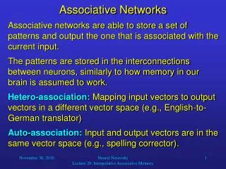
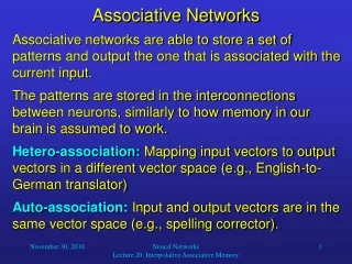
1. Associative Networks • Associative networks are able to store a set of patterns and output the one that is associated with the current input. • The patterns are stored in the interconnections between neurons, similarly to how memory in our brain is assumed to work. • Hetero-association: Mapping input vectors to output vectors in a different vector space (e.g., English-to-German translator) • Auto-association: Input and output vectors are in the same vector space (e.g., spelling corrector). Neural Networks Lecture 20: Interpolative Associative Memory

2. Interpolative Associative Memory • For hetero-association, we can use a simple two-layer network of the following form: O1 O2 … OM I1 I2 … IN Neural Networks Lecture 20: Interpolative Associative Memory

3. Interpolative Associative Memory • Sometimes it is possible to obtain a training set with orthonormal (that is, normalized and pairwise orthogonal) input vectors. • In that case, our two-layer network with linear neurons can solve its task perfectly and does not even require training. • We call such a network an interpolative associative memory. • You may ask: How does it work? Neural Networks Lecture 20: Interpolative Associative Memory

4. Interpolative Associative Memory • Well, if you look at the network’s output function you will find that this is just like a matrix multiplication: Neural Networks Lecture 20: Interpolative Associative Memory

5. Interpolative Associative Memory • With an orthonormal set of exemplar input vectors (and any associated output vectors) we can simply calculate a weight matrix that realizes the desired function and does not need any training procedure. • For exemplars (x1, y1), (x2, y2), …, (xP, yP) we obtain the following weight matrix W: Note that an N-dimensional vector space cannot have a set of more than N orthonormal vectors! Neural Networks Lecture 20: Interpolative Associative Memory

6. Interpolative Associative Memory • Example: • Assume that we want to build an interpolative memory with three input neurons and three output neurons. • We have the following three exemplars (desired input-output pairs): Neural Networks Lecture 20: Interpolative Associative Memory

7. Interpolative Associative Memory • Then If you set the weights wmn to these values, the network will realize the desired function. Neural Networks Lecture 20: Interpolative Associative Memory

8. Interpolative Associative Memory • So if you want to implement a linear function RNRM and can provide exemplars with orthonormal input vectors, then an interpolative associative memory is the best solution. • It does not require any training procedure, realizes perfect matching of the exemplars, and performs plausible interpolation for new input vectors. • Of course, this interpolation is linear. Neural Networks Lecture 20: Interpolative Associative Memory

9. The Hopfield Network • The Hopfield model is a single-layered recurrent network. • Like the associative memory, it is usually initialized with appropriate weights instead of being trained. • The network structure looks as follows: X1 X2 … XN Neural Networks Lecture 20: Interpolative Associative Memory

10. The Hopfield Network • We will first look at the discrete Hopfield model, because its mathematical description is more straightforward. • In the discrete model, the output of each neuron is either 1 or –1. • In its simplest form, the output function is the sign function, which yields 1 for arguments  0 and –1 otherwise. Neural Networks Lecture 20: Interpolative Associative Memory

11. The Hopfield Network • For input-output pairs (x1, y1), (x2, y2), …, (xP, yP), we can initialize the weights in the same way as we did it with the associative memory: This is identical to the following formula: where xp(j) is the j-th component of vector xp, andyp(i) is the i-th component of vector yp. Neural Networks Lecture 20: Interpolative Associative Memory

12. The Hopfield Network • In the discrete version of the model, each component of an input or output vector can only assume the values 1 or –1. • The output of a neuron i at time t is then computed according to the following formula: This recursion can be performed over and over again. In some network variants, external input is added to the internal, recurrent one. Neural Networks Lecture 20: Interpolative Associative Memory

13. The Hopfield Network • Usually, the vectors xp are not orthonormal, so it is not guaranteed that whenever we input some pattern xp, the output will be yp, but it will be a pattern similar to yp. • Since the Hopfield network is recurrent, its behavior depends on its previous state and in the general case is difficult to predict. • However, what happens if we initialize the weights with a set of patterns so that each pattern is being associated with itself, (x1, x1), (x2, x2), …, (xP, xP)? Neural Networks Lecture 20: Interpolative Associative Memory

14. The Hopfield Network • This initialization is performed according to the following equation: You see that the weight matrix is symmetrical, i.e., wij = wji. We also demand that wii = 0, in which case the network shows an interesting behavior. It can be mathematically proven that under these conditions the network will reach a stable activation state within an finite number of iterations. Neural Networks Lecture 20: Interpolative Associative Memory

15. The Hopfield Network • And what does such a stable state look like? • The network associates input patterns with themselves, which means that in each iteration, the activation pattern will be drawn towards one of those patterns. • After converging, the network will most likely present one of the patterns that it was initialized with. • Therefore, Hopfield networks can be used to restore incomplete or noisy input patterns. Neural Networks Lecture 20: Interpolative Associative Memory

16. The Hopfield Network • Example: Image reconstruction • A 2020 discrete Hopfield network was trained with 20 input patterns, including the one shown in the left figure and 19 random patterns as the one on the right. Neural Networks Lecture 20: Interpolative Associative Memory

17. The Hopfield Network • After providing only one fourth of the “face” image as initial input, the network is able to perfectly reconstruct that image within only two iterations. Neural Networks Lecture 20: Interpolative Associative Memory

18. The Hopfield Network • Adding noise by changing each pixel with a probability p = 0.3 does not impair the network’s performance. • After two steps the image is perfectly reconstructed. Neural Networks Lecture 20: Interpolative Associative Memory

19. The Hopfield Network • However, for noise created by p = 0.4, the network is unable the original image. • Instead, it converges against one of the 19 random patterns. Neural Networks Lecture 20: Interpolative Associative Memory

20. The Hopfield Network • Problems with the Hopfield model are that • it cannot recognize patterns that are shifted in position, • it can only store a very limited number of different patterns. • Nevertheless, the Hopfield model constitutes an interesting neural approach to identifying partially occluded objects and objects in noisy images. • These are among the toughest problems in computer vision. Neural Networks Lecture 20: Interpolative Associative Memory