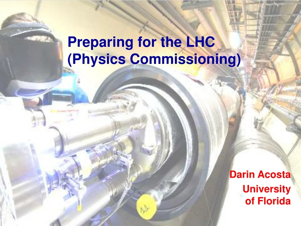
Preparing for the LHC (Physics Commissioning)
700 likes | 715 Views
This lecture discusses the scale of the commissioning problem, activities involved, test beam programs, detector performance, alignment, calibration, operating the experiment, data quality monitoring, and more.

Preparing for the LHC (Physics Commissioning)
E N D
Presentation Transcript
Preparing for the LHC (Physics Commissioning) Darin Acosta University of Florida Commissioning lecture 2 - HCP Summer School
Outline of Lectures • What is commissioning? • Scale of the problem • Detectors, electronics, software, computing • Commissioning activities • Test beam programs • Detector “Slice Tests” • Magnetic field measurements • Detector performance • Temporal alignment (synchronization) • Spatial alignment • Material budget • Calibration • Operating the Experiment • What it takes to run a large experiment • Data quality monitoring Lecture 1 Lecture 2 Lecture 3 Commissioning lecture 2 - HCP Summer School
Outline, Cont’d Lecture 3 • Preparing for physics measurements • Luminosity measurement & beam conditions • Impact of pile-up • Understanding the detector performance from data • Impact of instrumental issues (noisy/dead channels, zero suppression) on basic physics objects • Missing Transverse Energy – catch-all of instrumental problems • Jet Energy scale • Early LHC physics measurements • Underlying event • Calibrating the Standard Model backgrounds • e.g. QCD jet production, Electroweak measurements, Top quark measurements Lecture 4 Commissioning lecture 2 - HCP Summer School
Summary of Commissioning Exercises • You always learn something! • Expect the unexpected (electronics failures, detector noise, …) • It is important to test slices of the complete system for functionality (vertical slice tests), and the portions of the full system for scale (horizontal slice tests) • Because of the importance of the LHC turn-on, and the possibility of new discoveries right at the beginning, we are trying to pre-commission as much as we can before beams • But this implies trade-offs: • Commissioning exercises vs. installation activities • Global data-taking exercises vs. subsystem commissioning • It’s a “chicken-or-egg” problem: • If we wait for installation to be over, we have not pre-commissioned in time • We can’t commission until we are installed… Commissioning lecture 2 - HCP Summer School
Detector Performance Success in commissioning will be judged quantitatively by achieving the design performance from the detector subsystems Commissioning lecture 2 - HCP Summer School
First things first: Check the connections Commissioning lecture 2 - HCP Summer School
Synchronization Time-in your electronics Commissioning lecture 2 - HCP Summer School
Collisions @ CMS Beams cross every 25 ns Particles fly at v=c Detectors register hits at different absolute times Commissioning lecture 2 - HCP Summer School
Synchronization: General Picture • Synchronization means making fine delay adjustments to the electronics signals from the various detector components so that the data from a single beam crossing are received and processed in coincidence, despite different flight times • Need to time in: • The synchronous Level-1 trigger system so inputs are coincident • The capture of pulses for the data acquisition system (DAQ) based on the trigger signal • The time assignment & association of captured data (BX, event number) • There is one master reference clock that drives everything Channel 1 Channel 2 delay Commissioning lecture 2 - HCP Summer School
The Clock • Is the heartbeat of the experiment • Most of the front-end detector electronics and the Level-1 trigger electronics march to its beat • LHC bunch crossing frequency: 40.0788 MHz • Approximately 25 ns bunch crossing (BX) spacing • Since this is a very short interval, cannot complete the full Level-1 trigger decision within 1 BX (actually takes ~100) • Thus, the digital electronic systems are pipelined, with the clock synchronized (via phase-locked loops, PLLs) to the LHC frequency • Each clock edge marks the arrival of data from the next collision • Catastrophic error if the experiment clock is disrupted, or the frequency changes Commissioning lecture 2 - HCP Summer School
Dataflow of a synchronous digital electronic board (Level-1 Muon Track-Finding Board) • A complex task is partitioned into individual steps • Register output of each step so that data can be processed every BX even though entire operation takes >1BX Data moves to next step on each clock edge Optical link inputs provide track segments Track candidates output Data from 13 BX on board at any one time, latency: 13*25ns=0.33s Commissioning lecture 2 - HCP Summer School
Multiple boards, crates, racks • Single board is embedded within a system of many crates and racks of electronics Even the optical links connecting the detectors to the electronics add delays due to the finite speed of light, and hold many collisions (20 BX in this case) Commissioning lecture 2 - HCP Summer School
Level-1 Trigger Synchronization • For a synchronous system, one needs to add delays and adjust phases to keep data synchronized when collecting data from multiple boards (e.g. at the Global Trigger) • If not, you will be mixing up different events! • This can be tricky • There are a lot of boards! But some delays can be calculated (cables, logic) • Need to send periodic pulses to check time alignment, and look at the data itself for coincidences t Board 1: Board 2: Board 3: Board 4: Commissioning lecture 2 - HCP Summer School
Example of (mis)timed trigger electronics • Cosmic ray signals from muon detector trigger electronics Data coming late relative to trigger pulse Timed-in to trigger pulse Relative BX Commissioning lecture 2 - HCP Summer School
Signal Capture and Synchronization to Trigger • The analog pulses coming from the detectors must be delayed or otherwise stored, and then digitized (ADC, TDC) after a Level-1 trigger accept decision arrives • So timing-in the data acquisition electronics generally means capturing the data inside a certain time window defined relative to the trigger signal, with the clock phase adjusted so that the peak is in a fixed, desired position • Otherwise you are in danger of losing your detector signals, or misinterpreting the integral of the pulse (the charge) Reconstruction algorithms usually expect a fixed peak location, or shape Trigger pulse Time slices read out Commissioning lecture 2 - HCP Summer School
Adjusting phases of calorimeter signals • Adjusting the clock phase in 1ns steps to align pulse in window • One channel of CMS hadron calorimeter responding to laser pulse Peak is ½ clock later Peak is 1 clock later Commissioning lecture 2 - HCP Summer School
Synchronizing Event fragments • Once your trigger is synchronized, and pulses captured, one should ensure that the data captured by the DAQ actually corresponds to the same collision • Time markers include the Level-1 event number and the bunch crossing (BX) number • There could be a lot of interesting discoveries at the LHC if data fragments are not properly aligned! (e.g. momentum imbalance) Presumed invisible SUSY particle because data associated to wrong event! Dijet event becomes… Commissioning lecture 2 - HCP Summer School
LHC Bunch Structure (another handle) • 3564 “buckets” spaced 25ns apart span one LHC orbit • 2808 (80%) buckets to be filled with protons per LHC design • Structure of gaps provides a useful “fingerprint” to check synchronization of electronics Long”abort gap” Commissioning lecture 2 - HCP Summer School
Time alignment of BX structure • Accumulate data from each electronic channel and bin occurrences vs. BX number • Look for offsets in the fingerprint, then adjust delays or counters to match channel 1 channel 2 t Commissioning lecture 2 - HCP Summer School
Bunch Crossing Structure Example • For example, the SPS provided a testbeam with bunches synchronized to the LHC frequency (48 BX train) • CMS muon detector electronics (cathode strip chambers) exhibited this structure during 2004 tests 924 BX 48 BX BX Commissioning lecture 2 - HCP Summer School
Synchronization with particles • Of course to achieve synchronization requires some particles! • Three possible sources of particles for synchronizing detectors in-situ in the collision hall: • Cosmic ray muons (all we have at the moment…) • Asynchronous (random), and with asymmetric time-of-flight timing • Beam halo particles (single beam or collision operation) • Synchronous with 25ns bunch spacing, but asymmetric time-of-flight timing • Collision particles • Synchronous with 25ns bunch spacing, nominal timing • The first two have biases, thus we need LHC collisions to complete the synchronization of the detectors Commissioning lecture 2 - HCP Summer School
Cosmic ray timing (asymmetric) tup–tdown<0 Commissioning lecture 2 - HCP Summer School
Beam halo (asymmetric) tright-tleft <0 Commissioning lecture 2 - HCP Summer School
Collision particle timing tup–tdown~ 0tright-tleft ~0 Commissioning lecture 2 - HCP Summer School
Spatial Alignment Commissioning lecture 2 - HCP Summer School
Why alignment? • Efficiency of associating correct detection “hits” to a charged particle’s trajectory depends on proper understanding of detector alignment (for severe displacements) • Even more importantly, the assignment of the momentum of a charged particle via its curvature in a magnetic field depends on the precise alignment • pT = q B r , q=charge, B= magnetic field, r=radius • So we must align our detectors to get optimum performance for physics measurements X X X X R1 R2 R1 X X Commissioning lecture 2 - HCP Summer School
PT Resolution • Study of effect on PT resolution due to misalignment of CMS Tracker Commissioning lecture 2 - HCP Summer School
What needs to be measured • For every active detector element, 6 degrees of freedom: • Translation vector r = (x, y, z) • Rotation angles (, , ) • Store this in geometry file used by reconstruction software Actual position z’ z y’ y x x’ r Nominal position Commissioning lecture 2 - HCP Summer School
Survey • First step is to survey theplacement of your installeddetector elements • Positioning of detector modules or chambers (collections of individual sensor elements) • Deviates from nominal position by placement accuracy, gravity, magnetic forces, … • Complemented by careful measurements of the detector internal geometry during construction phase as well • Positioning of individual strips, cells, towers within a module • This can be very accurate for some systems Commissioning lecture 2 - HCP Summer School
Survey Surveyor Newly installed CMS electromagnetic calorimeter (half-barrel) inside solenoid Commissioning lecture 2 - HCP Summer School
Photogrammetry(Or why do I get those bright spots when I take a flash picture?) • Photogrammetry is the determination of 3D geometry from photographic images (taken at various angles) of pre-positioned reflective targets • Precision of survey and photogrammetry data can reach 300m (0.3mm) even for large objects Picture taken of a complete disk of CMS cathode strip chambers (muon detectors) – 2 alignment pins per chamber Commissioning lecture 2 - HCP Summer School
Optical alignment systems • To monitor changes in the detector alignment due to changing conditions (temperature, magnetic field), need dedicated optical systems • Precision down to ~100m • Along with survey/photogrammetry information, optical alignment information is complementary to information from in-situ track-based alignment (next topic) • Can remove some invariants of the problem Commissioning lecture 2 - HCP Summer School
CMS Muon Barrel Alignment system • LED+laser sources with precision distance and angle sensors • Position and orientation of 250 chambers 3000 d.o.f. • 4000 measurements Commissioning lecture 2 - HCP Summer School
Measured distortion of endcap iron disks • Test of alignment system during test of CMS 4T solenoid • 15mm inward “bow” of 1000 ton disk by 10g magnetic force! Measurements FEA calculations Commissioning lecture 2 - HCP Summer School
Laser Alignment System extends into Inner Tracker Commissioning lecture 2 - HCP Summer School
Track-based alignment • Align sensors using in-situ tracks • Generally yields the ultimate precision, O(10m) for tracking • Requires data • General principle: • Every track has a series of measurements in detector sensors that we are interested in aligning to better precision • Take the residual difference between the measured position and the fitted track trajectory for each hit on the track and for all tracks • Minimize the sum of the squared residuals, normalized by the measurement error, over all hits and all tracks by adjusting the alignment parameters • The problem: • The number of modules to align, N, is very large • N=15K for CMS strip tracker, 6 d.o.f., 100K alignment parameters! • Computationally intensive (but solvable!) Commissioning lecture 2 - HCP Summer School
Some details • Ignoring correlations between measurements and dependence on track parameters (q) • Which generally implies that one iterates the minimization procedure several times with the position information improved from the previous calculation • Minimize function to solve for alignment corrections • Generally the solution involves solving a large matrix equation, which is block diagonal 6N x 6N Commissioning lecture 2 - HCP Summer School
Approaches to solve problem • Exactly solving the full matrix equation (i.e. inverting a large matrix) only feasible for O(1000-10000) parameters • CPU time goes as N3, memory as N2 • MILLEPEDE algorithm (V.Blobel) does that (since 1996) • Has been used successfully for tracking alignment at the H1 experiment (vertex detector and drift chamber), as well as at CDF, HERA-b, and LHC-b • To solve higher-dimensional matrices (100K), need to go to iterative procedures • e.g. MILLEPEDE-2, started 2005, but also: • Hits and Impact Points algorithm (HIP) • V. Karimaki, A. Heikkinen, T. Lampen, and T. Linden – works with only 6x6 matrix blocks rather than inverting full 6N x 6N • Kalman filter approach • R. Fruhwirth, E. Widl, and W. Adam – updates alignment information after each track is processed Commissioning lecture 2 - HCP Summer School
HIP alignment demonstration on CMS Pixels • 720 pixel barrel modules, assuming strip tracker aligned • Monte Carlo study of 200K Z0 ~25m stand-alone pixels Commissioning lecture 2 - HCP Summer School
Tracker Alignment: Cosmic Muons at CMS TIF • First alignment results on small data sample (50K events) from the CMS Tracker Integration Facility • Only HIP algorithm used so far • Recall about 20% of strip tracker instrumented • TIB residual: ~600 μm with no alignment, ~170 μm after 30 iterations • 30 hours, 3.6 GHz Xeon dual CPU • Analysis ongoing with moredata, and other algorithms Iteration 0 Iteration 3 Iteration 20 Commissioning lecture 2 - HCP Summer School
Demonstration of alignment of Complete CMS Tracker! Monte Carlo study, MILLEPEDE-2. Strips and Pixels together L ~ 0.5 fb-1 Results better than foreseen Pixels RMS to 2m or better Commissioning lecture 2 - HCP Summer School
Why cosmic muons, beam halo muons, and other constraints are necessary • The track-based alignment methods have some invariants using only one class of tracks, i.e. particles coming from interaction point • Some deformations leave the 2 sum invariant • Need tracks atother angles to solve these ambiguities Commissioning lecture 2 - HCP Summer School
Despite all that precision, don’t forget to check the actual installed geometry! • Sometimes large, but subtle, effects such as the symmetry in the offset staggering of detectors can be missed ! • A pure Monte Carlo simulation and reconstruction would have been self consistent • But analyzing real data with the coded reconstruction geometry can point out problems • Other examples: • Which side of the cavern the shaft is located • Where the “chimney” is for the cryogenic pipes i.p. even-numbered chambers odd-numbered chambers Commissioning lecture 2 - HCP Summer School
Material Budget Commissioning lecture 2 - HCP Summer School
Material Budget • Along with knowing where everything is, it also helps to know just how much of everything you have! • Reason: the tracking system must meet contradictory goals of having sensors to measure particle trajectories whilst using as little material as possible to minimize scattering, which would disturb the measurement • In addition, precision electron and photon measurements benefit from minimizing the material in front of the calorimeter, which otherwise will cause • Electrons to bremsstrahlung (causes poor energy measurement) • Photons to convert (causes electron fakes) • At a minimum, one needs to know how much material is there to simulate its effects • Historically, experiments get this wrong a priori and significantly underestimate the amount of material • Hard to know where every cable and pipe is that gets installed Commissioning lecture 2 - HCP Summer School
Estimated CMS Tracker Material Budget • X0 = radiation length • Electron radiates all but e-1 = 37% of its energy in 1X0 • Mean free path of photons is 9/7 X0 Commissioning lecture 2 - HCP Summer School
Methods to Measure Material in Data • Weigh the components of your built detector and services (pipes, supports, etc.) and compare with the “weight” in your geometry model used by simulation and reconstruction • e.g. CMS has a systematic campaign for the final Strip Tracker to measure this to accuracy < 10% • Measure processes sensitive to the material budget, e.g. • Electrons will radiate photons due to the material in their path • Measure amount of bremsstrahlung • Photons (from 0 for example) will convert (pair produce e+e-) • Measure fraction of converted photons e e+ e- Commissioning lecture 2 - HCP Summer School
CMS Electron Reconstruction • Uses a type of track reconstruction called “Gaussian Sum Filter” • Ability to associate silicon tracker hits to trajectory even with bremsstrahlung all the way to the ECAL • More hits attached better measurement • Provides momentum measurement at vertex (before bremsstrahlung) and at outer radius of helix (after) • Ratio of Pin/Pout indicates bremsstrahlung • Classification of electrons based on this Different classes Occurence in Clustered energy over true Commissioning lecture 2 - HCP Summer School
Material budget from electrons • Since exp(-X/X0) is fraction of energy not radiated (1-fbrem) • X/X0 = - ln (1 – fbrem) • So measuring this quantity from electrons on average gives the material budget distribution (statistical accuracy ~2%) • Tracks changes in budget; tracks true value, with some scaling Commissioning lecture 2 - HCP Summer School