Multiple linear regression
Multiple linear regression. Tron Anders Moger 11.10.2006. Example:. Repetition: Simple linear regression. We define a model where are independent, normally distributed, with equal variance

Multiple linear regression
E N D
Presentation Transcript
Multiple linear regression Tron Anders Moger 11.10.2006
Repetition: Simple linear regression • We define a model where are independent, normally distributed, with equal variance • Wish to fit a line as close to the observed data (two normally distributed varaibles) as possible • Example: Birth weight=β0+β1*mother’s weight
How to compute the line fit with the least squares method? • Let (x1, y1), (x2, y2),...,(xn, yn) denote the points in the plane. • Find a and b so that y=a+bx fit the points by minimizing • Solution: where and all sums are done for i=1,...,n.
How do you get this answer? • Differentiate S with respect to a og b, and set the result to 0 We get: This is two equations with two unknowns, and the solution of these give the answer.
How close are the data to the fitted line? R2 • Define • SSE: Error sum of squares • SSR: Regression sum of squares • SST: Total sum of squares • We can show that SST = SSR + SSE • Define • R2 is the ”coefficient of determination”
Example: Regression of birth weight with mother’s weight as independent variable
Interpretation: • Have fitted the line Birth weight=2369.672+4.429*mother’s weight • If mother’s weight increases by 20 pounds, what is the predicted impact on infant’s birth weight? 4.429*20=89 grams • What’s the predicted birth weight of an infant with a 150 pound mother? 2369.672+4.429*150=3034 grams
But how to answer questions like: • Given that a positive slope (b) has been estimated: Does it give a reproducible indication that there is a positive trend, or is it a result of random variation? • What is a confidence interval for the estimated slope? • What is the prediction, with uncertainty, at a new x value?
Confidence intervals for simple regression • In a simple regression model, • a estimates • b estimates • estimates • Also, where estimates variance of b • So a confidence interval for is given by
Hypothesis testing for simple regression • Choose hypotheses: • Test statistic: • Reject H0 if or
Prediction from a simple regression model • A regression model can be used to predict the response at a new value xn+1 • The uncertainty in this prediction comes from two sources: • The uncertainty in the regression line • The uncertainty of any response, given the regression line • A confidence interval for the prediction:
Example: The confidence interval of the predicted birth weight of an infant with a 150 pound mother • Found that the predicted weight was 3034 grams • The confidence interval for the prediction is: 2369.67+4.43*150±t187,0.025*1.71*√(1+1/189+(150-129.81)2/(175798.52)) • Which becomes (3030.8, 3037.5) =1.96
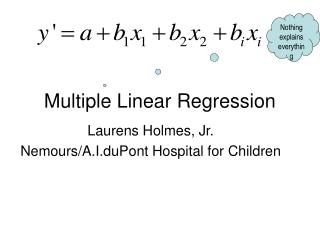
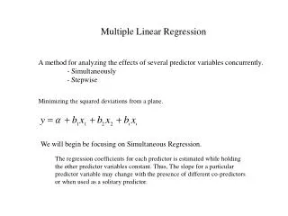
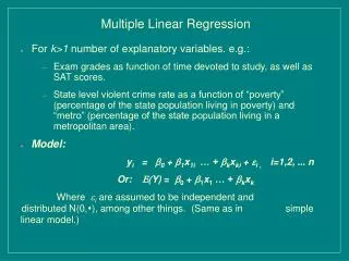
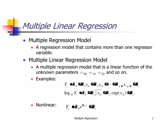
More than one independent variable: Multiple regression • Assume we have data of the type (x11, x12, x13, y1), (x21, x22, x23, y2), ... • We want to ”explain” y from the x-values by fitting the following model: • Just like before, one can produce formulas for a,b,c,d minimizing the sum of the squares of the ”errors”. • x1,x2,x3 can be transformations of different variables, or transformations of the same variable
Multiple regression model • The errors are independent random (normal) variables with expectation zero and variance • The explanatory variables x1i, x2i, …, xni cannot be linearily related
New example: Traffic deaths in 1976 (from file crash on textbook CD) • Want to find if there is any relationship between highway death rate (deaths per 1000 per state) in the U.S. and the following variables: • Average car age (in months) • Average car weight (in 1000 pounds) • Percentage light trucks • Percentage imported cars • All data are per state
Univariate effects (one independent variable at a time!): Deaths per 1000=a+b*car age (in months) • Hence: If all else is equal, if average car age increases by one month, you get 0.062 fewer deaths per 1000 inhabitants; increase age by 12 months, you get 12*0.062=0.74 fewer deaths per 1000 inhabitants Deaths per 1000=a+b*car weight (in pounds)
Univariate effects cont’d (one independent variable at a time!): Hence: Increase prop. light trucks by 20 means 20*0.007=0.14 more deaths per 1000 inhabitants Predicted number of deaths per 1000 if prop. Imported cars is 10%: 0.206-0.004*10=0.17
Building a multiple regression model: • Forward regression: Try all independent variables, one at a time, keep the variable with the lowest p-value • Repeat step 1, with the independent variable from the first round now included in the model • Repeat until no more variables can be added to the model (no more significant variables) • Backward regression: Include all independent variables in the model, remove the variable with the highest p-value • Continue until only significant variables are left • However: These methods are not always correct to use in practice!
For the traffic deaths, end up with: • Deaths per 1000=2.7-0.037*car age +0.006*perc. light trucks Conclusion: Did a multiple linear regression on traffic deaths, with car age, car weight, prop. light trucks and prop. imported cars as independent variables. Car age (in months, β=-0.037, 95% CI=(-0.063, -0.012)) and prop. light trucks (β=0.006, 95% CI=(0.004, 0.009)) were significant on 5%-level
Least squares estimation • The least squares estimates of are the values b1, b2, …, bK minimizing • They can be computed with similar but more complex formulas as with simple regression
Explanatory power • Defining • We get as before • We define • We also get that Coefficient of determination
Adjusted coefficient of determination • Adding more independent variables will generally increase SSR and decrease SSE • Thus the coefficient of determination will tend to indicate that models with many variables always fit better. • To avoid this effect, the adjusted coefficient of determination may be used:
Drawing inference about the model parameters • Similar to simple regression, we get that the following statistic has a t distribution with n-K-1 degrees of freedom: where bj is the least squares estimate for and sbj is its estimated standard deviation • sbj is computed from SSE and the correlation between independent variables
Confidence intervals and hypothesis tests • A confidence interval for becomes • Testing the hypothesis vs • Reject if or
Testing sets of parameters • We can also test the null hypothesis that a specific set of the betas are simultaneously zero. The alternative hypothesis is that at least one beta in the set is nonzero. • The test statistic has an F distribution, and is computed by comparing the SSE in the full model, and the SSE when setting the parameters in the set to zero.
Making predictions from the model • As in simple regression, we can use the estimated coefficients to make predictions • As in simple regression, the uncertainty in the predictions has two sources: • The variance around the regression estimate • The variance of the estimated regression model
What if the relationship is non-linear: Transformed variables • The relationship between variables may not be linear • Example: The natural model may be • We want to find a and b so that the line approximates the points as well as possible
Example (cont.) • When then • Use standard formulas on the pairs (x1,log(y1)), (x2, log(y2)), ..., (xn, log(yn)) • We get estimates for log(a) and b, and thus a and b
Another example of transformed variables • Another natural model may be • We get that • Use standard formulas on the pairs (log(x1), log(y1)), (log(x2), log(y2)), ...,(log(xn),log(yn)) Note: In this model, the curve goes through (0,0)
A third example: • Assume data (x1,y1),..., (xn,yn) seem to follow a third degree polynomial • We use multivariate regression on (x1, x12, x13, y1), (x2, x22, x23, y2),... • We get estimated a,b,c,d, in a third degree polynomial curve
Doing a regression analysis • Plot the data first, to investigate whether there is a natural relationship • Linear or transformed model? • Are there outliers which will unduly affect the result? • Fit a model. Different models with same number of parameters may be compared with R2 • Check the assumptions! • Make tests / confidence intervals for parameters • A lot of practice is needed!
Conclusion and further options • Regression versus correlation: • Can include more independent variables in regression • Gets a more detailed picture on the effect a independent variable has on the dependent variable • What if the dependent variable only has two possible values? Logistic regression • Similar to linear regression • But the interpretations of the β’s are different: They are interpreted as odds-ratios instead of the slope of a line

