Succession Model
Succession Model. We talked about the facilitation, inhibition, and tolerance models, but all of these were verbal descriptions Today we are going to consider a mathematical model that describes those processes more precisely and generates predictions that can be tested in the real world.

Succession Model
E N D
Presentation Transcript
Succession Model • We talked about the facilitation, inhibition, and tolerance models, but all of these were verbal descriptions • Today we are going to consider a mathematical model that describes those processes more precisely and generates predictions that can be tested in the real world
Succession Model • To do this, we will develop a matrix model of ecological succession that describes in general terms, the ways in which communities change from one “state” to another through time • We can also set of the parameters of the model to describe the processes of facilitation, inhibition, and tolerance
Succession Model • We will a Markov model to predict changes in populations and communities • Initially we need to define a number of mutually exclusive stages that represent different, discrete communities • These stages may represent entire sets of species (e.g. algal mats, encrusting sponges), or they could even represent individuals or stands of a single species (e.g. red oak)
Succession Model • When organizing and classifying communities into discrete stages, it may be necessary to make some decisions about stages
Succession Model • When choosing the stages for the model implicitly sets the spatial scale of the patch • For example, if the stages represent individual species, then a single patch must not be so large as to hold more than one species at a time • In addition, there may need to be a open space stage (following a disturbance)
Succession Model • Remember, all stages must be independent and in your model, all possible stages must be accounted for
Succession Model • Specifying the Time Step • Once stages are established, the investigator must specify the time step of the model • We will use a discrete time step (hence will not need to use differential equations) • This may be years, decades, or days/weeks
Succession Model • Constructing the Stage Vector • Suppose we have n possible stages for a patch and the landscape consists of a large number of such patches • We can then create a stage vector that tells us the number of patches in each of the stages
Succession Model • Consider a landscape with 4 patch types: open space, grassland, shrub, and forest • If we censused 500 patches we might have the following: s(t) = [250,100,80,70] • (t) indicates the stage vector at time t • 0’s are possible as some stages may not be represented • We can now predict changes through time
Succession Model • Constructing the Transition Matrix • The transition matrix is slightly different than some other matrices (e.g. Leslie) in both the possible values entered and the interpretation • If there are n stages in our model, the transition matrix A will be square, with n rows and n columns
Succession Model • Each column of matrix represents the patch state at the current time (t), and each row represents the patch state at the next time step (t+1). The entries are the transition probabilities for change from the current state (column) to the next stage (row)
Succession Model • Example of a typical matrix. The probability of moving from grassland (column) to the open state (row) is 0.23 and the probability of moving from forest to grassland is 0.10
Succession Model • The stage transitions are not necessarily symmetric. For example, although the probability of moving from grassland to the open state is 0.23, the probability of moving from the open state to grassland is 0.15. • The diagonals of the matrix indicate the probability that a patch remains in its current state and does not change
Succession Model • Probabilities of remaining in the same state are represented on the diagonals
Succession Model • This example points out some of the general properties of transition matrices for succession models. • First, notice that all of the entries are positive numbers between 0-1.0 (thus a probability). • Second, all values sum to 1.0 (we have included all possible states)
Succession Model • Loop Diagrams • The transition matrix can be represented by a loop diagram (a circle representing each stage) • Use a one-headed arrow to connect two stages
Succession Model • Loop diagram for the transition matrix
Succession Model • Projecting Community Change • The transition matrix summarizes all of the information on how patches change from one state to another • The matrix is a set of probabilistic ‘rules’ that determine the patterns of succession that will occur from any possible starting point
Succession Model • Using vector s at time t, we can use the transition matrix (A) to determine the number of patches in each state at the next time step (t+1) s(t+1) = As(t) • In this example, we had 100 patches in grassland at time t. How many will occur at time t+1?
Succession Model • There are four ways in which grassland patches can appear at time t+1: there can be transitions from open space, shrub, or forest and some grassland patches will remain grassland patches GP (t+1) = (0.15)(250) + (0.70)(100) + (0.25)(80) + (0.10)(70) = 134.5
Succession Model e.g. Grass Patches (t+1) = (0.15)(250) + (0.70)(100) + (0.25)(80) + (0.10)(70) = 134.5
Succession Model Remaining patches: OP(t+1)=(0.65)(250) + (0.23)(100) + (0.25)(80) + (0.40)(70) = 233.5 SP(t+1)=0(250)+(0.07)(100)+(0.25)(80)+(0.15)(0.40)(70) = 37.5 FP(t+1)=(0.2)(250)+0(100)+(0.25)(80)+(0.35)(70) = 94.5
Succession Model • So we started with the vector: s(0) = [250, 100, 80, 70] and after one time step, ended up with: s(1) = [233.5, 134.5, 37.5, 94.5] • Although the patch states changed, the total number of patches remains the same (500) • You can repeat and calculate t+2…
Succession Model • Determining the Equilibrium • Even though the content of the stage vector keeps changing, remember that the transition matrix A remains the same throughout the process. Consequently, in relatively short time the stage vector reaches an equilibrium state s(t) = [223.03, 164.7, 31.52, 80.75]
Succession Model • Once this equilibrium has been reached, there will be no further change in these numbers • Interestingly, the same equilibrium vector is reached irrespective of initial patch distribution
Succession Model • Successional trajectories for two initial patch vectors: a) [250 100 80 70] & [500 0 0 0]
Succession Model • Pg 193
Succession Model • Model Variations: Facilitation • We can utilize strategically placed 0’s in the matrix, which ensures that patches move through the sequence in orderly fashion
Succession Model • Idealized loop diagram for the facilitation model
Succession Model • Model Variations: Inhibition • In this model, we can assume that each of the 3 community states (grass, shrub, forest) can be replaced by another community state only through an intervening disturbance that frees up space
Succession Model • Consequently, stages can only remain as they are or go to the open stage (and then transition into any one of the others)
Succession Model • Idealized loop diagram for the inhibition model
Succession Model • Model Variations: Tolerance • For the tolerance model, assume that all states, including the open state, are equally likely. This generates a transition matrix with identical transition elements. • Each community neither inhibits nor facilitates replacement by other communities (therefore equally likely)
Succession Model • Notice the equal likelihood in the tolerance model
Succession Model • Idealized loop diagram for the tolerance model
Model Comparison • Patch trajectories for simple successional model. In each model the initial vector is s(0) = [1000 0 0 0] • The inhibition and tolerance matrices settle into their equilbria after a single time step (facilitation takes ~20 steps)
Succession Model • Empirical Examples: desert vegetation • Can get a good measure of the dynamic nature of desert vegetation (the slow decay allows for relatively good estimate of mortality and patch transition)
Succession Model • This matrix is not clearly any of the idealized matrices we have discussed thus far (e.g. Larreararely colonizes open space and the seedlings of Larrea are almost always found beneath Ambrosia.
Succession Model • This is a type of facilitation, although it does not lead to orderly species replacement as in the classic facilitation model (plus it takes a very long time between steps, a gradual replacement) • The diagonals are close to 1.0. So what?
Succession Model • It turns out the observed matrix matches the equilibrium stage vector relatively well • There is an underrepresentation ofLarrea(2.8%) compared to the predicted (9.9%), perhaps due to density-dependent mortality
Succession Model • Observed and expected frequencies of patch states
Succession Model • This model can be used to forecast how this desert community may respond to a human disturbance
Succession Model • Following severe human disturbance, it takes a very long time (~2000 yrs) to settle into equilibrium