Download
1 / 33
330 likes | 464 Views
Dipole Antennas Driven at High Voltages in the Plasmasphere. Linhai Qiu Mentor: Timothy Bell Advisor: Umran Inan December 12, 2010. Outline. Introduction Nonlinear Sheath Impedance Number Densities of Electrons and Ions Antenna Tuning The Effects of Ion-to-electron Mass Ratio Summary.

E N D
Dipole Antennas Driven at High Voltages in the Plasmasphere Linhai Qiu Mentor: Timothy Bell Advisor: Umran InanDecember 12, 2010
Outline • Introduction • Nonlinear Sheath Impedance • Number Densities of Electrons and Ions • Antenna Tuning • The Effects of Ion-to-electron Mass Ratio • Summary
Introduction • The plasma sheath characteristics have significant influence on the input impedance of antennas driven by high-voltages in magnetized plasmas. • Study the near-field properties of antennas driven by voltages from 86 V to 5000 V with AIP code developed by Timothy Chevalier. • Extracting accurate models of sheath capacitance and conductance from numerical results and developing the method of tuning high-voltage antennas in the plasmasphere.
Outline • Introduction • Nonlinear Sheath Impedance • Number Densities of Electrons and Ions • Antenna Tuning • The Effects of Ion-to-electron Mass Ratio • Summary
Simulation • Code: Fully parallel 3-D nonlinear multi-moment hydrodynamic code developed by Timothy Chevalier • Simulation object: Determine near field of antennas in the magnetosphere for various driving voltages. • To provide an example, consider the antenna located at L = 3 where the electron density is 1×10⁻⁹ m−3, the magnetic field is 1.165×10⁻⁶ T, the plasma temperature is 2000 K. The length of one antenna branch is 9 m, the gap between the two antenna elements is 2 m, the diameter of the antenna is 10 cm, and the frequency is 25 kHz.
Voltage at 103 V drive voltage • The voltage variation shown on the left is the voltage of one antenna element, defined to be the voltage with respect to the distant neutral plasma. • Maximum positive voltage: 10 V • Maximum negative voltage: -100 V
Conductive Current (103 V) • The currents shown on the left are the currents formed by the particles from the plasmas hitting on one antenna element. • Peak-to-peak magnitude: ~ 2 mA • Electron current has larger peak magnitude, but shorter duration • Proton current has smaller peak magnitude, but longer duration
Displacement Current (103 V) • The displacement currents shown on the left is defined as the derivative of the charge of one antenna element with respect to time. • Peak-to-peak magnitude: ~ 3 mA • Nonlinear and NOT sinusoidal • Conductive current is non-negligible compared to displacement current
Voltage at 1035 V drive voltage • Maximum positive voltage: 100 V • Maximum negative voltage: -950 V • It appears that there may be a small long-term variation of the average voltage. The cause of such variation is still under investigation.
Conductive Current (1035 V) • Peak-to-peak magnitude: ~ 10 mA • Peak-to-peak magnitude 5 times as large as that of 103 V • Indicating the sheath conductance decreases as the voltage increases
Displacement Current (1035 V) • Peak-to-peak magnitude: ~ 22.5 mA • Peak-to-peak magnitude 7.5 times as large as that of 103 V • Sheath capacitance decreases slower than sheath conductance as the voltage increases
Sheath Capacitance (86V) • The analytical model: Mlodnoskyand Garriott(1963) • Analytical model assumes protons are stationary • Analytical model gives sheath capacitance as coaxial cylindrical capacitance
Sheath Capacitance (1035 V) • The splitting occurs at low voltage magnitude
Sheath Conductance (86V) • The analytical model: derived based on the theory of metallic structures in gaseous discharges formulated by Mott-Smith and Langmuir [1926]
Sheath Conductance (1035 V) • The splitting occurs at low voltage magnitude • The figures contain the data points of 8 RF cycles • Inertia is the primary cause of splitting
Outline • Introduction • Nonlinear Sheath Impedance • Number Densities of Electrons and Ions • Antenna Tuning • The Effects of Ion-to-electron Mass Ratio • Summary
Evolution of Proton Number Density • 1 and 4 correspond to negative voltages • 2 and 3 correspond to positive voltages Antenna position: 30 m Antenna orientation: perpendicular to the magnetic field, vertical in the figure
Number Density of Particles ×109 8 Density / m-3 6 4 2 • Antenna position: 30 m • Antenna orientation: vertical 0 40 50 10 20 30 Position / m
Large Depletion Region Sheath region Depletion region • Distinguish depletion region from the sheath region • The depletion region outside sheath region is almost neutral • The shape of the depletion region is found to be roughly spherical by examining several slice planes
Outline • Introduction • Nonlinear Sheath Impedance • Number Densities of Electrons and Ions • Antenna Tuning • The Effects of Ion-to-electron Mass Ratio • Summary
Circuit model Need accurate models of sheath capacitance and sheath conductance
Extract New Models • Sheath capacitance • Add correction factors to the parameters of the original model • Minimizing least square errors numerically
Extract New Models • Sheath Conductance • Splitting is not reflected in the new models • Large errors at low voltages will not greatly influence the overall performance
Comparison at 103 V • After reaching the quasi-steady state, • Errors of peak-to-peak magnitude of the conductive currents: ~ 12 % • Errors of peak-to-peak magnitude of the displacement currents: ~ 12 %
Comparison at 1035 V • Errors are large in the transient response, but after reaching quasi-steady state, • Errors of peak-to-peak magnitude of the conductive currents: ~ 6 % • Errors of peak-to-peak magnitude of the displacement currents: ~ 1 % • The errors become smaller when the drive voltage is larger.
Tuning the Antenna • The left plot shows how the peak-to-peak charge magnitude on the antenna element changes with the value of tuning inductance L • Drive Voltage: 1500 V • Optimum inductance: 0.66 H • Maximum Charge: 680 nC
One Possible Tuning Scheme • Step 1: Calculate the real power and apparent power from the measured time domain v (t) and i (t) • Step 2: Calculate the reactive power Q from the apparent power S and the real power P according to the relation on the left. • Step 3: Estimate the change of tuning inductance needed to cancel the reactive power, so as to minimize the angle φ. • Step 4: Do tuning iteratively.
Mathematical Experiments • One example • Drive voltage: 1500 V • Optimum inductance: 0.66 H • Maximum charge: 0.68µC • Tuning process: • We will work with Ivan Galkin from UML to optimize the tuning scheme. 0H → 0.52 H → 0.71 H 0.19µC → 0.60µC → 0.65µC 43 mA → 107 mA → 113 mA
Outline • Introduction • Nonlinear Sheath Impedance • Number Densities of Electrons and Ions • Antenna Tuning • The Effects of Ion-to-electron Mass Ratio • Summary
Effects of Ion-electron Mass Ratio • Tim Chevalier used 200 as the proton-electron mass ratio to reduce the computation time. • The real mass ratio of proton to electron is 1835. • It can be predicted that both the proton and electron currents will decrease if using the mass ratio of 1835
Effects of Ion-electron Mass Ratio • Mass ratio mainly influences the conductive currents • The sheath capacitance and conductance model extracted at 86 V with 200 mass ratio correctly predicts the results at 1035 V with 1835 mass ratio
Summary • The efforts of modeling antenna-plasma coupling is extended to higher voltages that were not investigated before, from 86 V to 5000 V. The maximum voltage investigated by Timothy Chevalier was 86 V, due to the limited computer resources. • The terminal voltages, currents and input impedance of a dipole antenna in the plasmasphere are investigated from 86 V to 5000 V drive voltages with AIP code. • The particle number densities show a large quasi-neutral depletion regions surrounding the antenna elements • Models of conductance and capacitance of the sheath are extracted from the numerical results. • Tuning problems are investigated and an iterative tuning method is proposed and tested.