CSCI 4325 / 6339 Theory of Computation

1. CSCI 4325 / 6339Theory of Computation Zhixiang Chen Department of Computer Science University of Texas-Pan American

2. Chapter ThreeTuring Machines

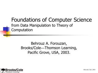
3. The Language Hierarchy of FA and PA • is not RL nor CFL. • But L is very simple and can be accepted by a simple program Regular Languages CF Languages

4. Δ a b a a … Read/write head Finite control Turing Machines (TM) Tape (input and working) Actions: Depending on its current symbol and current state, • Enter another state • Either - write a symbol - move read/write head one square right or left.

5. Formal Definition • A Turing machine is a quintuple: M = (K, , , S, H), where • K is a finite set of states •  is an alphabet, containing the blank symbol |_| and the left end symbol Δ, but not containing the symbols  and  • s  K is the initial state. • H  K is the set of halting states. • , the transition function, is a function from (K – H) X  to K X ( U {  , } ) such that: • (a)  q  K – H, if (q, Δ) = (p, b), then b =  • (b)  q  K – H and a , if (q, a) = (p, b) then b  Δ • Explain (q, a) = (p, b).

6. Examples • Consider M = (K, , , s, {h} ), where - What does this does? - Show examples.

7. Examples • Consider M = (K, , , s, {h} ), where • What does this machine do? • Show examples.

8. Configurations • Definition. Given M = (K, , , s, H), a configuration of M is a member of • K X * X (* ( - {Ц} ) U {e} ) • Content of a configuration: • current state • read/write head position • all symbols to the left of the r/w head • all symbols to the right of the r/w head (may be empty)

9. Δ a a b a _ _ … Configuration Examples • Find a configuration for the following snap shot of the TM

10. Δ _ _ _ _ a _ … Configuration Examples • Find a configuration for the following snap shot of the TM

11. Δ _ a _ _ _ _ … Configuration Examples • Find a configuration for the following snap shot of the TM

12. A Simple Notation of Configurations • (q, a a b a) • the current state is q • the current string is aaba • the current symbol is the second a • The underline indicates the current symbol, or • The r/w head position • Want more examples?

13. The Yield Relation • Let TM M = (K, , , s, H). Consider two configurations • (q1, 1 a1 u1) and • (q2, 2 a2 u2) • where a1, a2, , then (q1, 1 a1 u1) | (q2, 2 a2 u2) if and only if, for some b U { , }, (q1, a1) = (q2, b) and either • b , 1 = 2, u1 = u2, a2 = b, • b = , 1 = 2 a2, and either • u2 = a1 u1 if a1  Ц or u1  e or • u2 = e, if a = Ц and u1 = e • b =  , 2 = w1 a1, and either • u1 = a1 u2, or • u1 = u2 = e, and a2 = Ц

14. Cases of Yield Relation • Let , u *, where u does not end with a Ц, and let a, b . • Case 1: (q1, a) = (q2, b) • Example: • (q1 ,  a u) | (q2, b u) • Case 2: (q1, a) = (q2, ) • Example • (q1, bau) | (q2, bau)

15. Cases of Yield Relation • Case 3: (q1, a) = (q2, ) • Example: • (q1, abu) | (q2, abu) • (q1, a) | (q2, aЦ)

16. The Closure of Yield Relation • Let |* the reflexive transitive closure of | • | describes one step of computation of TM M • |* describes a sequence of zero or a finite number steps of computation of TM M • In other words, a computation by M is a sequence of configurations for some such that • the length of the computation is n or we write

17. Example • Δ table is given below • ( , Δaaaa) | • Finish the above computation.

18. Basic TM Machines • Symbol-writing machines: • a  U {, } – {Δ} is defined as follows: • if a , then writes a and then halts • if a  {, }, then moves r/w head according to the direction of a and then halt.

19. Better Notations • a = , for a , a-writing machine • Write an a • R = , right-moving machine, • move one square right • L = , left-moving machine • move one square left.

20. a b Combining Rules Semantics: Start at the initial state of M1; operate as M1 would operate until M1 would halt; then if the current symbol is a, start M2; otherwise if the current symbol is b, start M3.

21. a b R Δ |_| a, b, Δ, |_| R R TM Construction Examples • Examples 1 R

22. |_| L R R L |_| |_| TM Construction Examples • Example 2 |_|

23. Џ Џ L R R L Џ Џ TM Construction Examples • Example 3

24. The Copying Machine C • If C starts with input w, which contains only nonblank symbols but possibly empty and is put on an otherwise blank tape with one blank square to its left, and the head is put on the blank square to the left of w, then the machine C will eventually stop with w Ц w on an otherwise blank tape. We say that C transforms • Цω Ц into Ц ω Цω Ц

25. R a ≠ Џ Џ Џ Џ L Џ The Left-Shift Machine • S transforms • Ц w Ц to w Ц, where w is a nonblank string ЏL a R

26. a R Џ The a-Erasing Machine • This machines erase the a’s in its input tape

27. Computing with TM’s • Input representation of a TM M = (K, , , s, H) • Given  ( - {Ц, Δ })*, the input representation is Δ Ц  • The initial configuration is (s, ΔЦ)

28. Definitions • Let M = (K, , , s, H), H = {y, n} • Accepting configurations: Any halting configuration with the halting state y. • Rejecting configurations: Any halting configuration with the halting state n. • M accepts  if (s, Ц) yields an accepting configuration • M rejects  if (s, Ц) yields a rejecting configuration

29. Definitions • Let  =  - {, Ц} be the input alphabet. Given a language over  , M decides L if the following is true: * , • M accepts w if and only if  L. • A language L * is recursive if and only if there is a TM M that decides L. 0 0 0 0

30. b, d d a, d a b c d R R d R d L Џ c, Џ b, c Џ a, Џ y Examples • The language is recursive • Recall that L is not regular nor CF. • Construct a TM to accept Џ n

31. Recursive Functions TM’s as computing device • Definition: Let M = (K, , , s, H), 0 =  - { , Ц}, let * . Suppose that M halts on input , and that • (s, ΔЦ) | (h, Цy) for some y * . Then y is called the output of M on input , and is denoted as M(). • M() is defined if and only if M halts on . • In other words, (s, Ц) | (h, Цy) for some h  H and y *. 0 0

32. Recursive Functions TM’s as computing device • Let be a function. A TM M computes f if and only if • A function is recursive if and only if there is a TM computing f.

33. Examples • The doubling function d : * * such that •  w  , d() =  • d is recursive • The following TM computes d • C S • First make a copy of w to get w_w from _w , and then shift the copy to form _ww

34. Computing Numeric Functions • Coding natural numbers • Any natural numbers can be represented as strings in • {0} U {1, 2, …, 9} {0,1, 2, 3, …9}* or as strings • in {0} U {1} {0, 1}*

35. Definition. • Let M = (K, , δ, s, H) be a TM such that 0, 1, ; , and let f be any function We say that M computes f if • is recursive if there is a TM computing f.

36. 0 1 Џ 0 1 Џ 1 S R Example • The successor function is recursive. • The following TM computes the function: R L

37. Recursively Enumerable Languages • Note: A TM can be viewed as one of the three: • Acceptor • Computer • Generator • Definition. Let M = (K, , , s, H) be a TM, let 0 = - {, Ц} be an alphabet, and let L  be a language. We say that M semidecides L if for any string  the following is true: •  L if and only if M halts on input .

38. Recursively Enumerable Languages • A language L is r.e. if and only if there is a TM which semidecides L. • When M does not halt on input , we write • M () = • L is r.e. if and only if •  , M () =  L.

39. a R Examples • L = { {a, b}* :  contains at least one a } is r.e. • The following TM M semidecides L:

40. Recursive vs. R.E. Languages • Theorem. If a language is recursive, then it is r.e. • Theorem. If a language is recursive, then so is its complement. • Theorem: A language L is recursive if L and L are both r.e. • Proofs? (Prove in class)

41. … … … Extensions of TM • Multiple tapes

42. Definition of Multiple Tape TM • Definition. Let be an integer. A k-tape TM M is (K, , , s, H), where • K is the set of states •  is the set of input symbols • s K is the initial state • H  K is the set of final states. •  transition function, • Explain

43. Configurations of Multiple Tape TM • Definition. Let M=(K, , , s, H) be a k-tape TM. A configuration of M is a member of • Explain

44. The Yield Relation of k-Tape TM • Define the yield relation • Define the reflexive transitive closure of the yield relation • Accepting configurations? • Rejecting? • Copmputing? • R.e.?

45. Computing with a k-Tape TM • A k-tape TM can be used to compute a function or decide or semidecide a language. • Convention: • The first tape is the input and output tape • The other tapes are just working tapes. • K-tape TM’s are relatively easier to construct in some cases than single-tape TM’s

46. Example • Ex. Design a 2-tape TM to make a copy of the input: • Idea of construction • Copy ω to the second tape • Cope the content of the second tape to the first tape

47. Single Tape vs. Multiple Tapes • Theorem. Let M=(K, , , s, H) be a k-tape TM for some . Then there is a standard single tape TM M’=(K’, ’, ’, s’, H’) with  ’ such that the following holds:

48. Δ a _ b a _ _ Δ _ Δ b b b _ _ _ 0 0 1 0 0 0 0 Δ b b b _ _ _ 0 0 0 1 0 0 0 Δ a _ b a _ _ Proof. • Use 2k-tracks on a single-tape to simulate k-tape computation: • Each of the k-tapes can be simulated by two tracks: • One track for the content • The other track for the head position • Example

49. Corollary • Corollary. Any function that is computed or language that is decided or semidecided by a k-tape TM is also computed, decided, or semidecided, respectively by a standard single-tape TM.

50. Other Extensions of TM’s • Two-way infinite tape TM’s • Multiple heads TM’s • Two-dimensional tape TM’s • Random Access TM’s • Many other models … • All models have the same computational power • That is, for any two models, one model can do something, so does the other; and vice versa.