Download
1 / 33
330 likes | 447 Views
AIAA 2002-5531 OBSERVATIONS ON CFD SIMULATION UNCERTAINTIES. Serhat Hosder, Bernard Grossman, William H. Mason, and Layne T. Watson Virginia Polytechnic Institute and State University Blacksburg, VA Raphael T. Haftka University of Florida Gainesville, FL

E N D
AIAA 2002-5531OBSERVATIONS ON CFD SIMULATION UNCERTAINTIES Serhat Hosder, Bernard Grossman, William H. Mason, and Layne T. Watson Virginia Polytechnic Institute and State University Blacksburg, VA Raphael T. Haftka University of Florida Gainesville, FL 9th AIAA/ISSMO Symposium on Multidisciplinary Analysis and Optimization 4-6 September 2002 Atlanta, GA
Introduction • Computational fluid dynamics (CFD) as an aero/hydrodynamic analysis and design tool • CFD being used increasingly in multidisciplinary design and optimization (MDO) problems • CFD results have an associated uncertainty, originating from different sources • Sources and magnitudes of the uncertainty important to assess the accuracy of the results
Motivation • Design uncertainties due to computational simulation error • Optimization is an iterative procedure subject to convergence error. • Estimating convergence error may require expensive accurate optimization runs • Many simulation runs are performed in engineering design. (e.g., design of experiments) • Statistical analysis of error
Objectives • Find error characteristics of a structural optimization of a high speed civil transport • Estimate error level of the optimization procedure • Identify probabilistic distribution model of the optimization error • Estimate mean and standard deviation of errors without expensive accurate runs • Improve response surface approximation against erroneous simulation runs via robust regression
High Speed Civil Transport (HSCT) 250 passenger aircraft, 5500 nm range, cruise at Mach 2.4 Take off gross weight (WTOGW) is minimized Up to 29 configuration design variables including wing, nacelle and fuselage geometry, fuel weight, and flight altitude For this study, a simplified 5DV version is used
Structural optimization of HSCT For each HSCT configuration, wing structural weight (Ws) is minimized by structural optimization (GENESIS) with 40 design variables Structural optimization is performed a priori to build a response surface approximation of Ws
Effects of initial design point on optimization error • For Case 2, the initial design point was perturbed from that of Case 1, by factors between 0.1 ~ 1.9 • In average, Case 2 has the same level of error as Case 1 • The errors were calculated with respect to higher fidelity runs with tightened convergence criteria
Estimating error of incomplete optimization • To get optimization error we need to know true optimum, which is rarely known for practical engineering optimization • Optimization error = OBJ* - OBJ*true • To estimate OBJ*true • Find convergence setting to achieve very accurate optimization • This approach can be expensive
The Weibull distribution model • Widely used in reliability models (e.g., lifetime of devices) • Characterized by a shape parameter and a scale parameter PDF function according to
Estimation of distribution parameters • Maximum likelihood estimation (MLE) to estimate distribution parameters of the assumed distribution. • Find to maximize the likelihood function. • 2goodness of fit test • Comparison of histograms between data and fit • p-value indicates quality of the fit
h(t; 2) PDF g(s; 1) s, t x=s-t Difference fit to estimate statistics of optimization errors Errors of two optimization runs of different initial design point s = W1 – Wt t = W2 – Wt , (Wt is unknown true optimum.) The difference of s and t is equal to W1 – W2 x = s – t = (W1 – Wt) – (W2 – Wt ) = W1 – W2 We can fit distribution to x instead of s or t. • s and t are independent • Joint distribution of g(s) and h(t) • MLE fit for optimization difference x using f(x) • No need to estimate Wt
Comparison between error fit and difference fit • Difference fit is applied to the differences between Cases 1 and 2, assuming the Weibull model for both cases • Even when only inaccurate optimizations are available, difference fit can give reasonable estimates of uncertainty of the optimization
Estimated distribution parameters • Another set of optimization with a difference initial design point was enough, which is straightforward and no more expensive • The difference fit gave error statistics as accurate as the error fits involving expensive higher fidelity runs
Outliers and robust regression • Robust regression techniques • Alternative to the least squares fit that may be greatly affected by a few very bad data (outliers) • Iteratively reweighted least squares (IRLS) • Inaccurate response surface approximation is another error source in design process • Improve response surface approximation by repairing outliers
Iteratively Reweighted Least Squares Weighted least squares: Initially all points have same weight of 1.0. At each iteration, the weight is reduced for points that are far from the response surface. This gradually moves the response surface away from outliers. IRLS approximation leaves out detected outliers 1 dimensional example
Nonsymmetric weighting function • Regular weighting functions • Symmetrical • Huber’s function gives non-zero weighting to big outliers • Biweight rejects big outliers completely • Nonsymmetric weighting function • make use of one-sidedness of error by penalizing points of positive residual more severely Weighting functions of IRLS Aggressive search by reducing tuning constant B
Improvements of RS approximation by outlier repair Comparison of RS before and after repair
Drag polar results from 1st AIAA Drag Prediction Workshop (Hemsch, 2001)
Objective of the Paper • Finding the magnitude of CFD simulation uncertainties that a well informed user may encounter and analyzing their sources • We study 2-D, turbulent, transonic flow in a converging-diverging channel • complex fluid dynamics problem • affordable for making multiple runs • known as “Sajben Transonic Diffuser” in CFD validation studies
Transonic Diffuser Problem Weak shock case (Pe/P0i=0.82) P/P0i experiment CFD Strong shock case (Pe/P0i=0.72) P/P0i streamlines Separation bubble Contour variable: velocity magnitude
Uncertainty Sources (following Oberkampf and Blottner) • Physical Modeling Uncertainty • PDEs describing the flow • Euler, Thin-Layer N-S, Full N-S, etc. • boundary conditions and initial conditions • geometry representation • auxiliary physical models • turbulence models, thermodynamic models, etc. • Discretization Error • Iterative Convergence Error • Programming Errors We show that uncertainties from different sources interact
Computational Modeling • General Aerodynamic Simulation Program (GASP) • A commercial, Reynolds-averaged, 3-D, finite volume Navier-Stokes (N-S) code • Has different solution and modeling options. An informed CFD user still “uncertain” about which one to choose • For inviscid fluxes (commonly used options in CFD) • Upwind-biased 3rd order accurate Roe-Flux scheme • Flux-limiters: Min-Mod and Van Albada • Turbulence models (typical for turbulent flows) • Spalart-Allmaras (Sp-Al) • k- (Wilcox, 1998 version) with Sarkar’s compressibility correction
Grids Used in the Computations Grid 2 y/ht A single solution on grid 5 requires approximately 1170 hours of total node CPU time on a SGI Origin2000 with six processors (10000 cycles) Grid 2 is the typical grid level used in CFD applications
Nozzle efficiency Nozzle efficiency (neff ), a global indicator of CFD results: H0i : Total enthalpy at the inlet He : Enthalpy at the exit Hes : Exit enthalpy at the state that would be reached by isentropic expansion to the actual pressure at the exit
Discretization Error by Richardson’s Extrapolation error coefficient order of the method grid level a measure of grid spacing
Error in Geometry Representation Upstream of the shock, discrepancy between the CFD results of original geometry and the experiment is due to the error in geometry representation. Downstream of the shock, wall pressure distributions are the same regardless of the geometry used.
Downstream Boundary Condition Extending the geometry or changing the exit pressure ratio affect: • location and strength of the shock • size of the separation bubble
Uncertainty Comparison in Nozzle Efficiency Strong Shock Weak Shock Maximum value of
Conclusions • Based on the results obtained from this study, • For attached flows without shocks (or with weak shocks), informed users may obtain reasonably accurate results • They may get large errors for the cases with strong shocks and substantial separation • Grid convergence is not achieved with grid levels that have moderate mesh sizes (especially for separated flows) • Difficult to isolate physical modeling uncertainties from numerical errors
Conclusions • Uncertainties from different sources interact, especially in the simulation of flows with separation • The magnitudes of numerical errors are influenced by the physical models (turbulence models) used • Discretization error and turbulence models are dominant sources of uncertainty in nozzle efficiency and they are larger for the strong shock case • We should asses the contribution of CFD uncertainties to the MDO problems that include the simulation of complex flows