Statistical Learning
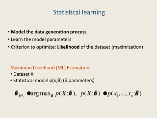
Statistical Learning. Inductive learning comes into play when the distribution is not known. Then, there are two basic approaches to take. Generative or Bayesian (indirect) Learning model the world and infer the classifier Discriminative (direct) learning

Statistical Learning
E N D
Presentation Transcript
Statistical Learning • Inductive learning comes into play when the distribution is not known. • Then, there are two basic approaches to take. Generative or Bayesian (indirect) Learning model the world and infer the classifier Discriminative (direct) learning model the classifier *directly* • A third non-statistical approach learns a discriminant function f:XY without using probabilities • Our COLT PAC studies apply generally CS446-Fall ’06
Generative / Discriminative Example • There are two coins: • a fair coin (P(Head) = 0.5) • a biased coin (P(Head) = 0.6) Coin 1 Coin 2 CS446-Fall ’06
Probabilistic Learning • There are actually two different probabilistic notions.(this is NOT the generative/discriminative distinction) • Learning probabilistic concepts • The learned concept is a function c:X[0,1] • c(x) may be interpreted as the probability that the label 1 is assigned to x • The learning theory that we have studied before is applicable (with some extensions) • Use of a probabilistic criterion in selecting a hypothesis • The hypothesis can be deterministic, a Boolean function, etc. CS446-Fall ’06
Probability Review • Sample Space - • Random Variable - • Probability Distribution – • Event - W: Set of possible worlds, Universe of atomic events (possibly infinite),… F: W R; Function mapping W to a range of values, vocabulary for W D: a [0,1] Measure over W with D({})=0, D(W)=1, D(a b)= D(a) + D(b) - D(a b)Watch out for the overloading of “D” distribution, [training] data A subset of W CS446-Fall ’06
Probability Review Example A (possibly biased) coin is flipped ten times What is the sample space? Is it finite or infinite? {Heads,Tails}10 or {0,1}10 so, finite Give a/the random variable. Give it’s domain. How many random variables are there? F1: the outcome of the first flip F2: the outcome of the second flip… to F10 NH: the total number of heads in the sequence lots – whatever aspects interest us F1, F2, F3, F4…F10 are different random variables that are iid (meaning?) “independent identically distributed” CS446-Fall ’06
Probability Review Two events, a and b are independent. Which best captures this? b b b a a a b Several of them All of them None of them a a b CS446-Fall ’06
Probability Review A is a random variable, a is one of its values; also for B & bP(A) is a distribution, P(a) or P(A=a) is a probability • P(a | b) = P(a b) / P(b) definition of conditional or posterior probability • P(a b) = P(a | b) * P(b) • P(a b) = P(a) + P(b) - P(a b) • P(A) = P(A,bi) marginalization B CS446-Fall ’06
Basics of Bayesian Learning • Goal: find the best hypothesis from some space H of hypotheses, given the observed data D. • Define best to be the most probable hypothesis in H • In order to do that, we need to assume a prior probability distribution over the class H. • In addition, we need to know something about the relation between the data observed and the hypotheses so that the training set can be interpreted as evidence for / against hypotheses. CS446-Fall ’06
Basics of Statistical Learning • P(h) - the prior probability of a hypothesis h Reflects background knowledge; before data is observed. If no information – often assume uniform distribution. • P(D) - The probability that this sample of the Data is observed. (No knowledge of the hypothesis) • P(D|h): The probability of observing the sample D, given that hypothesis h is the target • P(h|D): The posterior probability of h. The probability h is the target, given that D has been observed. CS446-Fall ’06
Bayes Theorem • P(h|D) increases with P(h) and with P(D|h) • P(h|D) decreases with P(D) • Easy to re-derive: multiply by P(D) CS446-Fall ’06
Learning Scenario • The learner considers a set of candidate hypotheses H (models), and attempts to find the most probable one h H, given the observed data. • Such maximally probable hypothesis is called maximum a posteriori hypothesis (MAP); Bayes theorem can be used to compute it: CS446-Fall ’06
Learning Scenario (2) • We may assume that a priori, hypotheses are equally probable • We get the Maximum Likelihood hypothesis: • Here we just look for the hypothesis that best explains the data CS446-Fall ’06
Examples • A given coin is either fair or has a 60% bias in favor of Head. • Decide what is the bias of the coin • Two hypotheses: h1: P(H)=0.5; h2: P(H)=0.6 • Prior: P(h): P(h1)=0.75 P(h2 )=0.25 • Now we need Data. 1stExperiment: coin toss is heads so D={H}. • P(D|h): P(D|h1)=0.5 ; P(D|h2) =0.6 • P(D): P(D)=P(D|h1)P(h1) + P(D|h2)P(h2 ) = 0.5 0.75 + 0.6 0.25 = 0.525 • P(h|D): P(h1|D) = P(D|h1)P(h1)/P(D) = 0.50.75/0.525 = 0.714 P(h2|D) = P(D|h2)P(h2)/P(D) = 0.60.25/0.525 = 0.286 CS446-Fall ’06