Product Curves

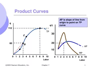
1. C 20 60 B 1 10 9 0 2 3 4 5 6 7 8 0 1 2 3 4 5 6 7 8 9 10 Labor Labor Product Curves AP is slope of line from origin to point on TP curve q q/L 112 TP 30 AP 10 MP Chapter 7

2. Practice • Bridget's Brewery production function is given by • where K is the number of vats she uses and L is the number of labor hours. Does this production process exhibit increasing, constant or decreasing returns to scale? Holding the number of vats constant at 4, is the marginal product of labor increasing, constant or decreasing as more labor is used? Chapter 7

3. Solution • Multiplying the K and L by 2 yields: • we know the production process exhibits constant returns to scale. Holding the number of vats constant at 4 will still result in a downward sloping marginal product of labor curve. That is the marginal product of labor decreases as more labor is used. Chapter 7

4. Chapter 7 The Cost of Production

5. Measuring Cost:Which Costs Matter? • Accountants tend to take a retrospective view of firms’ costs, whereas economists tend to take a forward-looking view • Accounting Cost • Actual expenses plus depreciation charges for capital equipment • Economic Cost • Cost to a firm of utilizing economic resources in production, including opportunity cost Chapter 7

6. Measuring Cost:Which Costs Matter? • Economic costs distinguish between costs the firm can control and those it cannot • Concept of opportunity cost plays an important role • Opportunity cost • Cost associated with opportunities that are foregone or the value of the next best alternative use of a resource Chapter 7

7. Opportunity Cost • An Example • A firm owns its own building and pays no rent for office space • Does this mean the cost of office space is zero? • The building could have been rented instead • Foregone rent is the opportunity cost of using the building for production and should be included in the economic costs of doing business Chapter 7

8. Opportunity Cost • A person starting their own business must take into account the opportunity cost of their time • Could have worked elsewhere making a competitive salary • Accountants and economists often treat depreciation differently as well Chapter 7

9. Measuring Cost:Which Costs Matter? • Although opportunity costs are hidden and should be taken into account, sunk costs should not • Sunk Cost • Expenditure that has been made and cannot be recovered • Should not influence a firm’s future economic decisions Chapter 7

10. Sunk Cost • Firm buys a piece of equipment that cannot be converted to another use • Expenditure on the equipment is a sunk cost • Has no alternative use so cost cannot be recovered – opportunity cost is zero • Decision to buy the equipment might have been good or bad, but now does not matter Chapter 7

11. Prospective Sunk Cost • An Example • Firm is considering moving its headquarters • A firm paid $500,000 for an option to buy a building • The cost of the building is $5 million for a total of $5.5 million • The firm finds another building for $5.25 million • Which building should the firm buy? Chapter 7

12. Prospective Sunk Cost • Example (cont.) • The first building should be purchased • The $500,000 is a sunk cost and should not be considered in the decision to buy • What should be considered is • Spending an additional $5,250,000 or • Spending an additional $5,000,000 Chapter 7

13. Measuring Cost:Which Costs Matter? • Some costs vary with output, while some remain the same no matter the amount of output • Total cost can be divided into: • Fixed Cost • Does not vary with the level of output • Variable Cost • Cost that varies as output varies Chapter 7

14. Fixed and Variable Costs • Total cost of production equals the fixed cost (the cost of the fixed inputs) plus the variable cost (the cost of the variable inputs), or… • Short time horizon – most costs are fixed • Long time horizon – many costs become variable Chapter 7

15. Fixed Cost Versus Sunk Cost • Fixed cost and sunk cost are often confused • Fixed Cost • Cost paid by a firm that is in business regardless of the level of output • Sunk Cost • Cost that has been incurred and cannot be recovered Chapter 7

16. Measuring Costs • Marginal Cost (MC): • The cost of expanding output by one unit • Fixed costs have no impact on marginal cost, so it can be written as: Chapter 7

17. Measuring Costs • Average Total Cost (ATC) • Cost per unit of output • Also equals average fixed cost (AFC) plus average variable cost (AVC) Chapter 7

18. A Firm’s Short Run Costs Chapter 7

19. Determinants of Short Run Costs – An Example • Assume the wage rate (w) is fixed relative to the number of workers hired • Variable costs is the per unit cost of extra labor times the amount of extra labor: wL Chapter 7

20. Determinants of Short Run Costs – An Example • Remembering that • And rearranging Chapter 7

21. Determinants of Short Run Costs – An Example • We can conclude: • …and a low marginal product (MPL) leads to a high marginal cost (MC) and vice versa Chapter 7

22. Determinants of Short Run Costs • Consequently (from the table): • MC decreases initially with increasing returns • 0 through 4 units of output • MC increases with decreasing returns • 5 through 11 units of output Chapter 7

23. TC Cost ($ per year) 400 VC 300 200 100 FC 50 Output 0 1 2 3 4 5 6 7 8 9 10 11 12 13 Cost Curves for a Firm Total cost is the vertical sum of FC and VC. Variable cost increases with production and the rate varies with increasing and decreasing returns. Fixed cost does not vary with output Chapter 7

24. MC ATC AVC AFC Cost Curves Chapter 7

25. The line drawn from the origin to the variable cost curve: Its slope equals AVC The slope of a point on VC or TC equals MC Therefore, MC = AVC at 7 units of output (point A) TC P 400 VC 300 200 A 100 FC 1 2 3 4 5 6 7 8 9 10 11 12 13 Output Cost Curves for a Firm Chapter 7

26. Cost in the Long Run • In the long run a firm can change all of its inputs • In making cost minimizing choices, must look at the cost of using capital and labor in production decisions • Now: The firms’ long-run cost minimizing decision Chapter 7

27. Cost in the Long Run • Capital is either rented/leased or purchased • Assume Delta is considering purchasing an airplane for $150 million • Plane lasts for 30 years – economic depreciation for the plane = $5 million per year • If the firm had not purchased the plane, it would have earned interest on the $150 million (of 10%) • Forgone interest is an opportunity cost that must be considered also Chapter 7

28. Cost in the Long Run • User cost of capital, then, can be described as: • r = Depreciation Rate + Interest Rate • In our example, depreciation rate was 3.33% and interest was 10%, so • r = 3.33% + 10% = 13.33% Chapter 7

29. Cost Minimizing Input Choice • How does a firm select inputs to produce a given output at minimum cost? • Assumptions • Two Inputs: Labor (L) and capital (K) • Price of labor: wage rate (w) • The price of capital • r = depreciation rate + interest rate Chapter 7

30. Cost in the Long Run • The Isocost Line • A line showing all combinations of L & K that can be purchased for the same cost • Total cost of production is sum of firm’s labor cost, wL, and its capital cost, rK: C = wL + rK • For each different level of cost, the equation shows another isocost line Chapter 7

31. Cost in the Long Run • Rewriting C as an equation for a straight line: • K = C/r - (w/r)L • Slope of the isocost: • -(w/r) is the ratio of the wage rate to rental cost of capital. • This shows the rate at which capital can be substituted for labor with no change in cost Chapter 7

32. Choosing Inputs • We will address how to minimize cost for a given level of output by combining isocosts with isoquants • We choose the output we wish to produce and then determine how to do that at minimum cost • Isoquant is the quantity we wish to produce • Isocost is the combination of K and L that gives a set cost Chapter 7

33. Capital per year K2 A K1 Q1 K3 C0 C1 C2 Labor per year L3 L2 L1 Producing a Given Output at Minimum Cost Q1is an isoquant for output Q1. There are three isocost lines, of which 2 are possible choices in which to produce Q1. Isocost C2 shows quantity Q1 can be produced with combination K2,L2 or K3,L3. However, both of these are higher cost combinations than K1,L1. Chapter 7

34. Input Substitution When an Input Price Change • If the price of labor changes, then the slope of the isocost line changes, -(w/r) • It now takes a new quantity of labor and capital to produce the output • If price of labor increases relative to price of capital, then capital is substituted for labor Chapter 7

35. B K2 A K1 Q1 C2 C1 L1 L2 Input Substitution When an Input Price Change Capital per year If the price of labor rises, the isocost curve becomes steeper due to the change in the slope -(w/L). The new combination of K and L is used to produce Q1. Combination B is used in place of combination A. Labor per year Chapter 7

36. Cost in the Long Run • How does the isocost line relate to the firm’s production process? Chapter 7

37. Cost in the Long Run • The minimum cost combination can then be written as: • Minimum cost for a given output will occur when each dollar of input added to the production process will add an equivalent amount of output. Chapter 7

38. Cost in the Long Run • If w = $10, r = $2, and MPL = MPK, which input would the producer use more of? Chapter 7

39. Example • If MPL = 10, MPK = 5 and w= r = $10 • Which input should the firm increase/decrease usage? • What if w increased to $20? Chapter 7

40. Long Run VersusShort Run Cost Curves • Long-Run Average Cost (LAC) • Most important determinant of the shape of the LR AC and MC curves is relationship between scale of the firm’s operation and inputs required to minimize cost • Constant Returns to Scale • If input is doubled, output will double • AC cost is constant at all levels of output Chapter 7

41. Long Run Versus Short Run Cost Curves • Increasing Returns to Scale • If input is doubled, output will more than double • AC decreases at all levels of output • Decreasing Returns to Scale • If input is doubled, output will less than double • AC increases at all levels of output Chapter 7

42. Long Run Versus Short Run Cost Curves • In the long run: • Firms experience increasing and decreasing returns to scale and therefore long-run average cost is “U” shaped. • Source of U-shape is due to returns to scale instead of diminishing returns to a factor of production (labor) like the short-run curve • Long-run marginal cost curve measures the change in long-run total costs as output is increased by 1 unit Chapter 7

43. Economies and Diseconomies of Scale • Economies of Scale • Can double output for less than double the original cost • Diseconomies of Scale • Doubling the output costs more than twice the original cost • U-shaped LAC shows economies of scale for relatively low output levels and diseconomies of scale for higher levels Chapter 7

44. Long Run Costs • Increasing Returns to Scale • Output more than doubles when the quantities of all inputs are doubled • Economies of Scale • Doubling of output requires less than a doubling of cost • Why the difference: can have constant returns to scale but still have economies of scale: Chapter 7

45. Long Run Versus Short Run Cost Curves • We will use short and long run costs to determine the optimal plant size • We can show the short run average costs for 3 different plant sizes • This decision is important because once built, the firm may not be able to change plant size for a while Chapter 7

46. Long Run Cost with Economiesand Diseconomies of Scale Chapter 7

47. Long Run Cost withConstant Returns to Scale • What is the firm’s long run cost curve? • Firms can change scale to change output in the long run • The long run cost curve is the dark blue portion of the SAC curve which represents the minimum cost for any level of output • Firm will always choose plant that minimizes the average cost of production Chapter 7

48. Long Run Cost withConstant Returns to Scale • The long-run average cost curve envelops the short-run average cost curves • The LAC curve exhibits economies of scale initially but exhibits diseconomies at higher output levels Chapter 7

49. Production with Two Outputs – Economies of Scope • Many firms produce more than one product and those products are closely linked • Examples: • Chicken farm--poultry and eggs • Automobile company--cars and trucks • University--teaching and research Chapter 7

50. Production with Two Outputs – Economies of Scope • Advantages • Both use capital and labor • The firms share management resources • Both use the same labor skills and types of machinery Chapter 7