Download
1 / 72
890 likes | 1.67k Views
DARPA-ARO MURI. Multi-modal Adaptive Land Mine Detection Using Ground-Penetrating Radar (GPR) and Electro-Magnetic Induction (EMI) . Jay A. Marble and Andrew E. Yagle. METAL. PLASTIC. Outline. Application Overview 1.1 Data Collection 1.2 Metal and Plastic Landmines

E N D
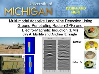
DARPA-ARO MURI Multi-modal Adaptive Land Mine Detection Using Ground-Penetrating Radar (GPR) and Electro-Magnetic Induction (EMI) Jay A. Marble and Andrew E. Yagle METAL PLASTIC
Outline • Application Overview • 1.1 Data Collection • 1.2 Metal and Plastic Landmines • 2. Sensor Phenomenology • 2.1 Ground Penetrating Radar (GPR) • 2.2 Electromagnetic Induction (EMI) • 2.3 Overview of Approach • 3. Metal Landmine Detection • 3.1 GPR Signature Features • 3.2 EMI Signature Features • 4. Plastic Landmine Detection • 4.1 Plastic Landmine Detection Difficulty • 4.2 Hyperbola Flattening Transform • 4.3 GPR Signature of Plastic Landmines • 4.4 Metal Firing Pin Detection • 5. Adapting to Changes in Environment • 6. Current Progress
1 2 3 4 5 6 7 9 8 10 11 12 13 14 15 16 1 3 5 7 13 9 15 17 11 19 2 4 6 10 12 8 14 16 18 20 1. Application Overview1.1 Data Collection USArmy Mine Hunter / Killer System EMI Coils GPR Antennae EMI Facts GPR Facts Bandwidth: 500MHz - 2GHz Operating: 75 Hz Frequency Sampling: Along Track: 5cm (2”) Cross Track: 15cm (6”) Swath: 3.0m Sampling: Along Track: 5cm Cross Track: 17.5cm Swath: 2.8m Depth Resolution: Free Space - 10cm (4”) Soil (er=3) - 5.7cm (2.3”) Database: 11000m2
1. Application Overview1.2 Metal Mines Metal Landmines Database Contains: 70 metal cased mines buried from 0” to 3” (Shallow). 93 metal cased mines buried from 3” to 6” (Deep). Type: TM-62M Metal Casing Burial Depth: 2” Width: 13” Height: 5.9” Type: M-15 Metal Casing Burial Depth: 3” Width: 13” Height: 5.9” M-21 Metal Casing Burial Depth: 1” Width: 13” Height: 8.1”
1. Application Overview1.2 Plastic Mines Plastic Landmines Type: TMA-4 Plastic Casing Burial Depth: 2” Width: 11” Height: 4.3” Type: TM-62P Plastic Casing Burial Depth: 2” Width: 13” Height: 5.9” Database Contains: 156 Shallow 265 Deep Type: VS1.6 Plastic Casing Burial Depth: 6” Width: 8.6” Height: 3.5” Type: VS2.2 Plastic Casing Burial Depth: 1” Width: 9” (.23m) Height: 4.5” (.115m) Type: M-19 Plastic Width: 0.33m Height: 3.5”
1. Application Overview GOAL: To determine presence vs. absence of land mines vs. other metal objects USING: Both GPR and EMI data (multi-modal detection algorithm) LANDMINES NOT LANDMINES How to discriminate between landmines and other objects using GPR and EMI ?
Outline • Application Overview • 1.1 Data Collection • 1.2 Metal and Plastic Landmines • 2. Sensor Phenomenology • 2.1 Ground Penetrating Radar (GPR) • 2.2 Electromagnetic Induction (EMI) • 2.3 Overview of Approach • 3. Metal Landmine Detection • 3.1 GPR Signature Features • 3.2 EMI Signature Features • 4. Plastic Landmine Detection • 4.1 Plastic Landmine Detection Difficulty • 4.2 Hyperbola Flattening Transform • 4.3 GPR Signature of Plastic Landmines • 4.4 Metal Firing Pin Detection • 5. Adapting to Changes in Environment • 6. Current Progress
Transmitted Frequencies f1 f2 fN Pulse Launch Sample Time 2.1 GPR Phenomenology Continuous, Stepped Frequency Radar 500MHz – 1.5GHz 128 Frequency Steps Tx Rx Antenna Module h Air Fourier Transform Transmit Pulse Ground Interface Layer 2 d Target ... Target f1 f2 fN f3 Sampled Frequencies Depth Profile [m]
2.1 GPR Phenomenology (echo from air-ground interface) (echo from buried target) • GT – Gain of transmit antenna • GR – Gain of receive antenna • ER – Electric field strength at the receiver • E0 – Transmitted Electric field strength. • h – Height of antenna above ground • d – Depth of target below the surface • – Wavelength in Free Space sRCS – Target Radar Cross Section (Propagation Constant Above the ground) *This model is for the antenna directly above the buried object.
2.1 GPR Phenomenology Slightly- Conducting Media Approximation
3 3 0 0 -3 -3 -6 -6 Depth [inches] -9 -9 Depth [inches] -12 -12 -15 -15 Simulated Data (“x-t” domain) -0.5 -0.5 0 0 0.5 0.5 1 1 Along Track [m] Along Track [m] - - - - Earth’s Surface x x Point Target (0,6”) (0,0.5) z z 2.1 GPR Phenomenology Data collected in time and space. Synthetic Aperture Antenna Pattern
2.1 GPR Phenomenology TM-62M Landmine Unimaged Signature TM-62M at 6” X Metal Casing Height: 6” Width: 13” Depth: 6” Z
Secondary Magnetic Field Source Air P r i m a r y M a g n e t i c F i e l d A i r G r o u n d Buried Sphere Ground 2.2 EMI Phenomenology Simplified EMI System Concept Current Source Data Storage Electronics & Sampler Source H-field Metal Object Reaction Incident Field at Object
Source Air Ground 2.2 EMI Phenomenology (x,y,h) (x,y,-d) Source H-field
Secondary Magnetic Field pz pr 2.2 EMI Phenomenology * Model assumes a solid spherical target. Metal Object Reaction
Induced Magnetic Sources pz px 2.2 EMI Phenomenology * Model no longer assumes a solid spherical target. Target Magnetic Polarizability Vector H0x – Horizontal magnetic field at the center of the target produced by the source magnetic dipole. Hxz – Vertical magnetic field at the receive coil produced by the horizontal induced magnetic dipole. H0z – Vertical magnetic field at the center of the target produced by the source magnetic dipole. Hzz – Vertical magnetic field at the receive coil produced by the vertical induced magnetic dipole.
2.2 EMI Phenomenology EMI Spatial Signature
2.2 EMI Phenomenology 1 2 3 4 5 6 7 8 9 10 11 12 13 14 15 16 EMI Spatial Signature Depth: 1” Depth: 3” Coil Number (Across Track) Along Track
Feature Extraction Stage Screener Stage Discriminant Stage Feature Vector 2.3 Overview of Approach POI Screener: Points-of-Interest (POI) are detected and reported. This stage must be fast and must detect all landmines, but can have false-alarms. Features: Aspects of the detected objects are characterized in a vector of feature values. Discriminant: Combines object features into a test statistic.
2.3 Overview of Approach: Screener Stage Point-of- Interest List
2.3 Overview of Approach: Feature Extraction POI List EMI Data EMI Data • Index X Location Y Location • 291456.6558 4227053.1692 • 2 291382.6225 4227053.3659 • 3 291354.7422 4227052.5429 • . • . • . • N 291309.1396 4227060.2448 4227052.5429 291354.7422 Feature Vector GPR Features Depth Width Height RCS EMI Features Magnetic Dipole Moments Decay Rates To Discriminant Function Extracted GPR Cube Extracted EMI Chip
Trained Statistic 2.3 Overview of Approach: Discriminant Function Quadratic Polynomial Discriminant Function (Shown here for 2 features.) • The QPD can be thought of as • a mapping. The feature vector • (x1,x2) is mapped into a statistic • “s” based on the training of the • coefficients (c1,c2,c3,c4,c5,c6). • The feature values are scalar • numbers describing object: • X1 - Feature Value 1 • (Like: object diameter) • X2 – Feature Value 2 • (Like: object depth) Output Statistic
Outline • Application Overview • 1.1 Data Collection • 1.2 Metal and Plastic Landmines • 2. Sensor Phenomenology • 2.1 Ground Penetrating Radar (GPR) • 2.2 Electromagnetic Induction (EMI) • 2.3 Overview of Approach • 3. Metal Landmine Detection • 3.1 GPR Signature Features • 3.2 EMI Signature Features • 4. Plastic Landmine Detection • 4.1 Plastic Landmine Detection Difficulty • 4.2 Hyperbola Flattening Transform • 4.3 GPR Signature of Plastic Landmines • 4.4 Metal Firing Pin Detection • 5. Adapting to Changes in Environment • 6. Current Progress
3. Metal Mines: Algorithm Adaptive Environmental Parameter Estimation EMI Data EMI Polarization Vector & Decay Rate EMI Simple Threshold Detection List Y/N W-k Imaging (Size/Depth) POI Detector GPR Data Discriminant Function Feature Extractor Proposed Architecture for Metal Landmine Detection
Focused Image 0.4 0.2 0 -0.2 -0.4 -0.6 -0.8 -1 -1.2 -1.4 -1.6 -1.5 -1 -0.5 0 0.5 1 1.5 After Azimuth FFT After Azimuth FFT After 2D Phase Compensation After 2D Phase Compensation (Kx,Kz) Domain after Stolt Interpolation (Kx,Kz) Domain after Stolt Interpolation 80 80 80 80 80 80 70 70 70 70 70 70 60 60 60 60 60 60 50 50 50 50 50 50 40 40 40 40 40 40 30 30 30 30 30 30 20 20 -60 -60 -40 -40 -20 -20 0 0 20 20 40 40 60 60 -60 -60 -40 -40 -20 -20 0 0 20 20 40 40 60 60 -60 -60 -40 -40 -20 -20 0 0 20 20 40 40 60 60 3. Wavenumber Migration Imaging Focused Point Target Mechanics of Wavenumber Migration Hyperbolic Point Target Place in W-k Format 2D Phase Comp. 2D FFT Stolt Interp. 2D Azimuth Stolt 2D Phase FFT Interp FFT Comp R(kx,W) R(kx,W)F(kx,,W) D(kx,kz)
3.1 GPR Signature TM-62M Landmine • Depth and Azimuth Resolution ere rrd variation medianinches Air 1 1 3.94 Dry Sand 4-6 5 1.76 Wet Sand 10-30 20 0.88 Dry Clay 2-5 3 2.27 Wet Clay 15-40 27 0.76 B = 1.5GHz f0 = 1.25GHz Q = 60° Metal Case Height: 6” Width: 13” Depth: 6”
3.1 GPR Signature Unimaged Signature • Signature before imaging • is dominated by the • standard hyperbola. • Depth can be determined • if data is properly • calibrated. Size requires • imaging to estimate. • “Convexity” of signatures • is determined by the • speed of propagation • in the medium. Depth [Inches] Along Track [Inches]
3.1 GPR Signature • Imaged signature shows • reflections from the top • and bottom of the • landmine. • Length of the object can now • be estimated from the • length of the top and • bottom reflections. • Height of the object can be • estimated from the distance • between the two reflections. • Depth has been calibrated • during the imaging process. Image Depth [Inches] Along Track [Inches]
3.1 GPR Signature Image • Estimated Depth and Size • Depth: 5.7” • Length: 11.3” • Height: 6.8” • Ground Truth • Depth: 6” • Length: 13” • Height: 6” 13” 6” Depth [Inches] Top Reflection Bottom Reflection (Dry Clay) Along Track [Inches] About 3 res. cells across target in depth.
3.1 GPR Signature Objects Reported • Four objects are identified • by setting a threshold and • clustering connected pixels. • Objects 1 and 2 are clearly • above the ground and can • be eliminated. • Objects 3 and 4 are the top • and bottom reflections. 2 1 3 Top Object 4 Depth [Inches] Bottom Object Along Track [Inches]
3.1 GPR Signature Objects Reported • Length is estimated by • averaging the lengths • of the two reflections. • (Est. Length: 11.3”) • Height is the distance • between the two • reflections. • (Est. Height: 6.8”) • Depth is the distance from • the ground surface (0”) • to the top reflection. • (Est. Depth: 5.7”) 10.8” 5.7” 6.8” Depth [Inches] 12.5” Along Track [Inches]
3.1 GPR Signature Repeatability Study Ten Signatures Before Imaging
3.1 GPR Signature Repeatability Study Ten Signatures After Imaging
3.1 GPR Signature Repeatability Study Ten Signatures Binarized
3.1 GPR Signature Length [inches] Height [inches] Depth [inches] Number Repeatability Study Note: Depth Sample Spacing: 1.1” Ground Truth: Depth: 6” Length: 13” Height: 6”
3.2 EMI Signature Magnetic Polarizability (signal model) (N Samples) (Least Squares Estimator) • To compute the H matrix, we must • know the depth of the target.
3.2 EMI Signature • GPR (Radar) gives depth information • EMI (Dipole models) give H matrix values • Combining these: Multi-modal detection • Synergy: Each helps the other work better
Induced Magnetic Sources pz px 3.2 EMI Signature
3.2 EMI Signature Aluminum Plate Iron Sphere Amps No Target Present Target Present time Decay Rate Discriminant
Aluminum Objects Iron Objects Normalized Response Time [ms] 3.2 EMI Signature • Sum of Decaying • Exponentials (Prony): • N=2 is usually enough • Decay Rate Features:
3. Metal Mines Summary GPR Features EMI Features • Magnetic Polarizability: • W-k Imaging Features: Depth Length Height • Decay Rate Features: • Other Features:
Outline • Application Overview • 1.1 Data Collection • 1.2 Metal and Plastic Landmines • 2. Sensor Phenomenology • 2.1 Ground Penetrating Radar (GPR) • 2.2 Electromagnetic Induction (EMI) • 2.3 Overview of Approach • 3. Metal Landmine Detection • 3.1 GPR Signature Features • 3.2 EMI Signature Features • 4. Plastic Landmine Detection • 4.1 Plastic Landmine Detection Difficulty • 4.2 Hyperbola Flattening Transform • 4.3 GPR Signature of Plastic Landmines • 4.4 Metal Firing Pin Detection • 5. Adapting to Changes in Environment • 6. Current Progress
4. Plastic Mines: Algorithm Proposed Architecture for Plastic Landmine Detection Adaptive Environmental Parameter Estimation EMI Data EMI (Firing Pin) HFT Detection Algorithm Detection List Y/N GPR Data W-k Imaging (Size/Depth) POI Detector Discriminant Function Feature Extractor
4.1 Plastic Mine Detection • The standard detection approach is to create the “plan view” image • below by taking a standard deviation over depth. • Using this statistic there are many false alarms, but most mines • are detected. Deeply buried plastic mines, however, are often missed. GPR Standard Detection Statistic – Standard Deviation Over Depth Bins
Background Statistics PDF Estimated from Histogram PDF Estimated from Histogram 3x10 3x10 3x10 3x10 - - - - 4 4 4 4 3x10 3x10 - - 3 3 4.1 Plastic Mine Detection
4.1 Plastic Mine Detection ROC Curve • About 80% of deep • VS1.6 plastic mines • are detectable. Probability of Detection Deeply Buried VS1.6 (Depth <3”) Probability of False Alarm
4.1 Plastic Mine Detection Surface Plastic Landmine (VS1.6) Top of Mine at 6” • Deeply buried plastic landmines face a low signal-to-noise ratio (SNR). • Strata in the ground can create large radar returns that lead to false alarms. • The Hyperbola Flattening Transform seeks to exploit all the “energy” of the hyperbolic signature. Soil Stratum
y 1/y 4.2 Hyperbola Flattening Mathematical Description Remapping: Original Hyperbola 45° Rotation Simulation Simulation Simulation Simulation • The Hyperbola Flattening Transform converts a hyperbolic • signature into a straight line at 45°.
4.2 Hyperbola Flattening 0° Application to Simulated Data • The RADON transform • creates “projections” by • summing along lines. • Projections are oriented • for 0° to 180°. 90° • Radon Transform of the • “flattened” hyperbola has a • strong maximum at 45° • corresponding to the “energy” • contained in the hyperbola. • Radon Transform illustration • shows a projection for 120° • from a circle. 120° 180°