Sample Selection Example
210 likes | 351 Views
This study investigates sample selection bias in wage estimation models using data generated from a simulated population. The analysis applies the Heckman selection model to correct for biases arising from missing data related to education and age. By comparing ordinary least squares (OLS) estimations with Heckman corrections, we observe how the coefficients for education and age differ under various conditions. The findings highlight the implications of selection bias on wage estimates and offer insights into effective model selection for accurate wage predictions.

Sample Selection Example
E N D
Presentation Transcript
Sample Selection Example Bill Evans
Draw 10,000 obs at random • educ uniform over [0,16] • age uniform over [18,64] • wearnl=4.49 + 0.08*educ + 0.012*age + ε • Generate missing data for wearnl
drawn from standard normal [0,1] • d*=-1.5+0.15*educ+0.01*age+0.15*z+v • wearnl missing if d*≤0 • wearn reported if d*>0 • wearnl_all=wearnl with non-missing obs.
εi and vi are assumed to be bivariate normal • E(εi) = E(vi) =0 • Var(εi) = σ2 • Var(vi) = 1 • Corr(εi,vi) = ρ • Cov(εi,vi) = ρ σ • In this case, ρ=0.25 and σ=0.46
Yi = β0 + β1educi + β2agei + εi • E[Yi | SSR] = β0 + β1educi + β2agei + E[εi | SSR] • E[εi | SSR] = E[εi | vi>-wiγ] = ρ σ φ(wiγ)/Φ(wiγ)
λi = φ(wiγ)/Φ(wiγ) • wiγ = γ0+educ γ1+age γ2+z γ3 • γ2 and γ3 are both constructed to be positive • cov(educ, λi) < 0 and • cov(age, λi) < 0
The omitted variable λi is negatively correlated with what is observed in the model • Therefore, the coefficients on educ and age in the selected sample will be too low
Numbe rof non-missing observations
OLS on all data (no missing obs) Generated by the equation wearnl=4.49 + 0.08*educ + 0.012*age + ε
OLS on reported data Smaller MSE Notice that the estimates for educ and age are now smaller
Probit, why is data non-missing Generated by the equation d*=-1.5+0.15*educ+0.01*age+0.15*z+v
Syntax for Heckman model in STATA . heckman wearnl educ age, select(educ age z); Equation of interest Variables in selection equation
Notice β’s have increased over OLS w/ missing data Cannot reject null Rho=0 Sigma right on Rho is a little off
Comparison of Estimates [% difference from OLS w/ all data]
* run heckman sample selection correction; • . * but use functional form to identify the model; • . heckman wearnl educ age, select(educ age);
Comparison of Estimates [% difference from OLS w/ all data]
