Basic QTL Analysis
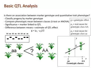
y. β o. 0. x. -1. aa. AA. Genotypic classes. Basic QTL Analysis Is there an association between marker genotype and quantitative trait phenotype? - Classify progeny by marker genotype - Compare phenotypic mean between classes (t-test or ANOVA)

Basic QTL Analysis
E N D
Presentation Transcript
y βo 0 x -1 aa AA Genotypic classes Basic QTL Analysis Is there an association between marker genotype and quantitative trait phenotype? - Classify progeny by marker genotype - Compare phenotypic mean between classes (t-test or ANOVA) - Significance = marker linked to QTL - Difference between means = estimate of QTL effect g = (µ1 - µ2)/2 g = genotypic effect µ1 = trait mean for genotypic class AA µ2 = trait mean for genotypic class aa
Notations for single-QTL models in backcross and F2 populations
Single-marker analysis • How it works • Finds associations between marker genotype and trait value • When to use • Order of markers unknown or incomplete maps • Quick scan • Find best possible QTLs • Identify missing or incorrectly formatted data • Limitations Underestimates QTL number and effects QTL position can not be precisely determined r = recombination fraction yj = trait value for the jth individual in the population μ = population mean f(A) = function of marker genotype εj = residual associated with the jth individual r A (marker) Q (putative QTL)
Single-marker analysis in backcross progeny • Parents: AAQQ x aaqq • Backcross: aaqq x AaQq x AAQQ Expected Frequency • BC Progeny AaQqAAQQ 0.5 (1 - r) AaqqAAQq 0.5r aaQqAaQQ 0.5r aaqqAaQq 0.5(1 - r) r is recombination frequency between A and Q
Single-marker analysis r A (marker) Q (putative QTL) • Simple t-test • Analysis of variance • Linear regression • Likelihood
Simple t-test using backcross progeny H0: [μAa - μaa ] = 0 (a + d) = 0 r = 0.5 Yj(i)k = μ + Mi + g(M)j(i) + ei(j)k Yj(i)k = trait value for individual j with genotype i in the replication k μ = population mean Mi = effect of the marker genotype g(M)j(i)= genotypic effect which cannot be explained by the marker genotype ei(j)k = error term µAa = trait mean for genotypic class Aa µaa = trait mean for genotypic class aa s2M = pooled variance within the two classes t-distribution with df = N – 2 If tM is significant, then a QTL is declared to be near the marker
Analysis of variance using backcross progeny H0: [μAa - μaa ] = 0 (a + d) = 0 r = 0.5 N= no. of individuals in pop. b = no. of replications r = recombination fraction F-distribution with 1 and N – 2 df If F is significant, then a QTL is declared to be near the marker F = t if df for numerator is 1
Analysis of variance using SAS (A simple example) data a; input Individuals Trait1 Marker1 Marker2; cards; 1 1.57 A B 2 1.35 B A 3 10.7 B B … proc glm; class Marker1 Marker2; model Trait1 = Marker1 Marker2; lsmeans Marker1 Marker2; run;
y βo x -1 aa Aa Genotypic classes 0 Linear regression using backcross progeny H0: [μAa - μaa ] = 0 (a + d) = 0 r = 0.5 R2: percent of the phenotypic variance explained by the QTL β1 Dummy variables: aa = -1 Aa = 1 yj= trait value for the jth individual xj= dummy variable βo= intercept for the regression β1= slope for the regression ej= random error Expectations: E(βo) = 0.5 (µAa + µaa) = Mean for the trait E(β1) = 0.5 (1 - 2r) (µAa - µaa) = (1 - 2r) g = 0.5 (a + d) (1 - 2r)
Linear regression using backcross progeny Interpretation of results depends on coding of the dummy variables y y x x aa aa Aa Aa Genotypic classes Genotypic classes µ = 3 µAa = 4 µaa = 2 g = 0.5(µAa - µaa) = 1 µ = 3 µAa = 2 µaa = 4 g = 0.5(µAa - µaa) = -1
A likelihood approach using backcross progeny Joint distribution function:
A likelihood approach using backcross progeny (cont.) (Weller, 1986) G-statistics Likelihood ratio test statistics (LR) Probability of occurrence of the data under the null hypothesis H0: [μAa - μaa ] = 0 (a + d) = 0 r = 0.5 G is distributed asymptotically as a chi-square variable with one degree of freedom The t-test is approximately equivalent to the likelihood ratio test using this formula
LOD score LOD : Logarithm of the odds ratio Base 10 logarithm of G LR= 2 (log)LOD = 4.605LOD LOD= 0.217LR LOD is interpreted as an odds ratio (probability of observing the data under linkage/probability of observing the same data under no linkage) No theoretical distribution is needed to interpret a lOD score Key value: ≥ 3 (H1 is 1000 times more likely than H0 -no linkage-) (approx: p = 0.001) p= probability of type I error Type I error: false positive (declare a QTL when there is no QTL)
Single-marker analysis Summary • Identify marker-trait associations • Identify missing or incorrectly formatted data • Genetic map is not required • Divide the population into subpopulations based on the allelic segregation of individual loci (one marker at a time) • Get trait means for each subpopulation (genotypic class) • Determine if the subpopulations trait means are significantly different • Limitations Underestimates QTL number and effects QTL position can not be precisely determined