Longitudinal Impedance Simulation of TDI in CST: All-Metal and Dielectric Components
590 likes | 715 Views
This document presents a comprehensive simulation of longitudinal impedance and wake fields for the TDI system using CST PS. The geometry includes all-metal and dielectric parts made from PEC, with no losses and excluding ferrites. Magnetic wall boundary conditions (BC) are applied at the horizontal plane, and PML BCs at the upstream and downstream ends with various mesh resolutions (σz) for accurate results. The report features impedance calculations across different beam locations and provides insights into the performance of hBN coatings and their resistivity.

Longitudinal Impedance Simulation of TDI in CST: All-Metal and Dielectric Components
E N D
Presentation Transcript
TDI longitudinal impedance simulation with CST PS Grudiev 20/03/2012
Geometry All metal and dielectric parts are from PEC. No losses. No ferrites are included. Magnetic wall BC is applied at the horizontal plane PML BCs are applied at the up/downstream ends
Different beam locations: b0, b1, b2 b2; X=-68mm b1; X=-8mm b0; X=0
Longitudinal Impedance, imaginary part, σz=100mm: b0, b1, b2 Half gap = 8mm b0: Z/n = 155 Ohm/250MHz * 400.8MHz/35640 = 7.0 mOhm b1: Z/n = 150 Ohm/250MHz * 400.8MHz/35640 = 6.7 mOhm b2: Z/n = 70 Ohm/200MHz * 400.8MHz/35640 = 3.9 mOhm
Longitudinal Impedance, real part, σz=100mm: b0, PML8 -> PML16 Almost no difference
Longitudinal Wake, σz=100mm: b0 beam pipe length: 200mm -> 100mm and 300mm
Longitudinal Impedance, σz=100mm: b0, beam pipe length 200mm -> 100mm and 300mm
Longitudinal Impedance, σz=100mm: b0, beam pipe length 200mm -> 100mm and 300mm Beam pipe length of 300 mm is better, but the difference is only at f ~ 0 And the negative offset of the ReZl is always there at the same level.
Ti coating of hBN blocks Dear all, Here is a coating report from Wil (please follow the link), for a batch of BN coated in 2010. The specifications we had been asked to meet were Rsquare<0.5 Ohm. For a thickness of about 5 µm that means a resistivity of about 250 e-8 Ohm.m , larger than the nominal Ti value. This is likely due to the large amount of outgassing from the porous BN material. Cheers, Sergio & Wil See EDMS link https://edms.cern.ch/document/1085514/1 For this coating skin depth in the range from 10 MHz to 1 GHz is 250 um to 25 um which is bigger than the coating thickness of 5 um.
Longitudinal Impedance, imaginary part, σz=100mm: b0, PEC hBN Half gap = 8mm b0, PEC: Z/n = 155 Ohm/250MHz * 400.8MHz/35640 = 7.0 mOhm b0, hBN: Z/n = 2620 Ohm/400MHz * 400.8MHz/35640 = 73.7 mOhm
Longitudinal Impedance, real part, : b0, hBN, σz=100 - > 50 mm
Longitudinal impedance gap 16mm hBN, withand w/o 4S60 NO DIFFERENCE
Longitudinal impedance gap 16mm hBN, σz = 100 mm , with and w/o Mask No big difference in CST wakefield solver BUT Saves a lot of mesh in HFSS eigenmode solver
Longitudinal impedance gap 16mm hBN, σz = 50 mm , with and w/o Mask No big difference in CST wakefield solver BUT saves a lot of mesh in HFSS eigenmode solver
R/Q estimate from PEC impedance Reminder from classical P. Wilson, SLAC-PUB-4547 For impedance of N modes with Q >> f/df, where df=c/s_max, for PEC Q~∞
R/Q estimated from longitudinal impedance, hBN, b0, σz = 50 mm 4(Zl-Zl0)*df/πf is plotted where Zl0 = 71 Ohm to make the real part positive