Download
1 / 72
720 likes | 744 Views
Dive into the world of digital signal processing with z-transforms and IIR-type discrete time filters. Learn about difference equations, recursive filters, frequency responses, and system functions. Explore how to find H(z) for various filter equations and implement signal flow graphs using MATLAB.

E N D
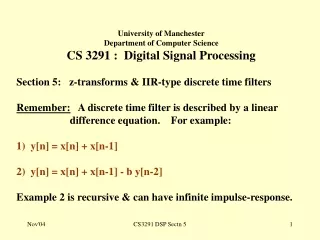
University of Manchester Department of Computer Science CS 3291 : Digital Signal Processing Section 5: z-transforms & IIR-type discrete time filters Remember: A discrete time filter is described by a linear difference equation. For example: 1) y[n] = x[n] + x[n-1] 2) y[n] = x[n] + x[n-1] - b y[n-2] Example 2 is recursive & can have infinite impulse-response. CS3291 DSP Sectn 5
Introduction: • General causal discrete time filter has difference equation: • N M • y[n] = a i x[n-i] - b j y[n-j] • i=0 j=1 • which is of order max{N,M}. • Recursive if any b j is non-zero. • A 2nd order recursive filter has the diff equn: • y[n] = a 0 x[n] + a 1 x[n-1] + a 2 x[n-2] - b 1 y[n-1] - b 2 y[n-2] • Frequency response of a discrete time filter:- • • H(e j ) = h[n]e - j n • n=- CS3291 DSP Sectn 5
Consider response of causal stable LTI system to {z n } • i.e. { …, z-2, z-1, 1, z, z2, z3, ……… } • By discrete time convolution, output is {y[n]} where • • y[n] = h[k] z n - k = z n h[k] z - k • k=- k=- • • = z n H(z) with H(z) = h[k] z - k • k=- • H(z) is "z-transform" of impulse-response. • Equivalent of Laplace transform. • H(z) is a complex number for any z. CS3291 DSP Sectn 5
For causal stable system, H(z) must be finite for z 1 • • H(z) = h[k] z - kh[k] z - k by causality • k=0 k=0 • • = h[k] z - k • k=0 • • h[k] when z 1 • k=0 • finite by defn of stability CS3291 DSP Sectn 5
Some properties of H(z): (1) H(z) is complex no. for any z with z1. (2) Replacing z by e j , gives H(e j ) rel frequency-resp. On Argand diagram ("z-plane"), z = e j lies on unit circle. (3) If input is {z n }, the output is {H(z) z n }. CS3291 DSP Sectn 5
System function is z-transform of {h[n]} : • • H(z) = h[k] z - n • n=- • Frequency-response is DTFT of {h[n]} : • • H(e j ) = h[n]e - j n • n=- • Replace z by e j CS3291 DSP Sectn 5
Example 5.1: Find H(z) for the non-recursive difference equation: y[n] = x[n] + x[n-1] Solution: {h[n]} = { ... , 0, 1, 1, 0, ... }, therefore H(z) = 1 + z - 1 CS3291 DSP Sectn 5
Example 5.2: Find H(z) for the recursive difference equation: • y[n] = a 0 x[n] + a 1 x[n-1] - b 1 y[n-1] • Solution: Method used above becomes hard. • Remember that if x[n] = z n then y[n] = H(z) z n , • y[n-1] = H(z) z n - 1 etc. • Substitute to obtain: • H(z) z n = a 0 z n + a 1 z n - 1 - b 1 H(z) z n - 1 • a 0 + a 1 z - 1 • H(z) = • 1 + b 1 z - 1 except when z = - b 1 . • When z = -b 1 , H(z) = . CS3291 DSP Sectn 5
For the general discrete time filter: • N M • y[n] = a i x[n-i] - b j y[n-j] • i=0 j=1 • the same method gives: • a 0 + a 1 z - 1 + a 2 z - 2 + ... + a N z - N • H(z) = • b 0 + b 1 z - 1 + b 2 z - 2 + ... + b M z - M • with b0 = 1. • Given H(z) in this form, we can easily get its difference equn • & hence its signal flow graph. CS3291 DSP Sectn 5
Example 5.3: Give a signal flow graph for: • a 0 + a 1 z -1 + a 2 z - 2 • H(z) = • 1 + b 1 z - 1 + b 2 z - 2 • Solution: The difference equation is: • y[n] = a 0 x[n] + a 1 x[n-1] + a 2 x[n-2] - b 1 y[n-1] - b 2 y[n-2] • Signal flow graph readily deduced. • Referred to as 2nd order or "bi-quadratic" IIR section • in "direct form 1". CS3291 DSP Sectn 5
Bi-quad IIR section in ‘direct form 1’ y[n] = a 0 x[n] + a 1 x[n-1] + a 2 x[n-2] - b 1 y[n-1] - b 2 y[n-2] CS3291 DSP Sectn 5
To implement this signal flow-graph as a program: a0 X Y z - 1 z -1 a1 - b1 X1 Y1 z - 1 z - 1 a2 - b2 X2 Y2 CS3291 DSP Sectn 5
In MATLAB using floating pt arithmetic: X1=0; X2=0; Y1=0; Y2=0; while 1 X = input(‘X=’); Y = a0*X + a1*X1 + a2*X2 - b1*Y1 - b2*Y2; disp(sprintf(‘Y = %f’ , Y) ) ; % output Y X2 = X1; X1 = X ; Y2 = Y1; Y1 = Y ; end; CS3291 DSP Sectn 5
In MATLAB using fixed pt arith & shifting: K=1024; A0=round(a0*K); A1=round(a1*K); A2=round(a2*K); B1=round(b1*K); B2=round(b2*K); X1=0; X2=0; Y1=0; Y2=0; while 1 X = input(‘X=’) ; Y = A0*X + A1*X1 + A2*X2 - A1*Y1 - A2*Y2 ; Y = round(Y/K); % Divide by arith right shift disp(sprint(‘Y=%f’,Y)); % Output Y X2 = X1; X1 = X ; % Prepare for next time Y2 = Y1; Y1 = Y ; end; CS3291 DSP Sectn 5
Alternative signal flow graphs: Re-order the two halves of Direct Form I Impulse response not changed (Problem 5.10). Simplify to : Direct Form II CS3291 DSP Sectn 5
"Direct Form II" signal flow graph:- It is a 2nd order (bi-quad) section whose system function is: a 0 + a 1 z -1 + a 2 z - 2 H(z) = 1 + b 1 z - 1 + b 2 z - 2 Its difference equation is:- y[n] = a 0 x[n] + a 1 x[n-1] + a 2 x[n-2] - b 1 y[n-1] - b 2 y[n-2] i.e. exactly the same as Direct Form 1 CS3291 DSP Sectn 5
Direct Form II has minimum no. of delay boxes. Example: Given values for a 1 , a 2 , a 0 , b 1 & b 2 , write program to implement Direct Form II using normal arithmetic. Solution: W1 = 0; W2 = 0; %For delay boxes while 1 X = input(‘X=’) ; % Input to X W =X - b1*W1 - b2*W2; % Recursive part Y = W*a0 + W1*a1 + W2*a2; % Non-rec. part W2 = W1; W1 = W; % For next time disp(sprintf(‘Y=%f’,Y)); % Output Y using disp end;% Back for next sample CS3291 DSP Sectn 5
% Direct Form II in fixed point arithmetic & shifting. K=1024; A0=round(a0*K); A1=round(a1*K); A2=round(a2*K); B1=round(b1*K); B2=round(b2*K); W1 = 0; W2 = 0; %For delay boxes while 1 X = input(‘X=’) ; % Assign X to input W =K*X - B1*W1 - B2*W2; % Recursive part W =round( W / K); % By arith shift Y = W*A0+W1*A1+W2*A2; % Non-rec. part W2 = W1; W1 = W; %For next time Y = round(Y/K); %By arith shift disp(sprintf( ‘Y=%f’, Y)); %Output Y using disp end;%Back for next sample CS3291 DSP Sectn 5
System function: • Expression for H(z) is ratio of polynomials in z - 1 . • Remove restriction z 1, & call H(z) "system function". • When z < 1 , H(z) need not be z-transform of {h[n]} • & need not be finite. • Nevertheless it is still useful to us. CS3291 DSP Sectn 5
Poles and zeros of H(z) • For a general discrete time filter:- • a 0 + a 1 z - 1 + a 2 z - 2 + ... + a N z - N • H(z) = • b 0 + b 1 z - 1 + b 2 z - 2 + ... + b M z - Mwith b0 = 1. • Re-express as: • (z N + a 1 z N -1 + ... + a N ) • H(z) = K z M - N • (z M + b 1 z M-1 + ... + b M )where K = a 0/b 0 • Factorise denom & numerator polynomials: • (z - z 1 )(z - z 2 )...( z - z N ) • H(z) = K z M - N • (z - p 1 )( z - p 2 )...(z - p M ) CS3291 DSP Sectn 5
So z 1 , z 2 ,..., z N, are "zeros". p 1 ,p 2 ,..., p M , are "poles”. • H(z) generally infinite with z equal to a pole. • H(z) generally zerowith z equal to a zero. • For a causal stable system: H(z) must be finite for z 1. • Cannot be a pole with modulus 1. • All poles must satisfy p i < 1. • On Argand diagram: poles must lie inside unit circle. • no restriction on the positions of zeros. CS3291 DSP Sectn 5
Gain response in terms of poles & zeros: • e j - z1e j - z2...ej - zN • H(e j ) = K • e j - p1e j - p2...e j - pM • Phase response: • Arg(H(e j )) = (M - N) + arg(e j - z 1 )+ ... + arg(ej - z N ) • - arg(e j - p1 ) - ... - arg(ej - p M) • On Argand diagram: e j - p1 is distance from p1 to e j • & Arg(e j - p1) is "pole angle" shown. • Similarly for e j - z1, e j - p2, etc. CS3291 DSP Sectn 5
Imag part of z exp(j) |ej- p| Arg(ej- p) P Real part of z Fig 5.5: z - plane CS3291 DSP Sectn 5
“Distance rule” Product distances from zeros to e j H(e j ) = K Product distances from poles to e j “Phase rule”: Arg(H(e j )) = (M-N) + sum of zero angles - sum of pole angles. CS3291 DSP Sectn 5
Example: Calculate gain-response of a filter with 1 + z - 1 H(z) = 1 - 1.273z - 1 + 0.81z - 2 Then plot poles & zeros of H(z) & comment on their effects: Before we start, please give (1) its difference equation & (2) its signal flow graph CS3291 DSP Sectn 5
x[n] y[n] z-1 z - 1 1.273 z - 1 -0.81 • Difference equation is: • y[n] = x[n] + x[n-1] + 1.273 y[n-1] - 0.81 y[n-2] • Signal flow graph in (Direct Form 1) is: CS3291 DSP Sectn 5
x[n] y[n] z-1 1.273 z-1 -0.81 • In Direct Form II, signal flow graph for:: • y[n] = x[n] + x[n-1] + 1.273 y[n-1] - 0.81 y[n-2] CS3291 DSP Sectn 5
Gain response: z (z + 1) This is H(z) = hard work! z 2 - 1.273 z + 0.81 [ e j W ] [1 + e j W ] H(e j ) = e 2 j - 1.273 e j W + 0.81 H(e j )2 = H(e j ) H * (e j ) = H(e j W) H(e - j W) [1 + e j ] [1 + e - j ] = [ e 2 j - 1.27 e j + 0.8] [ e - 2 j - 1.27 e - j + 0.81] 2 + 2 cos() = 3.28 - 4.61 cos() + 1.62 cos(2) CS3291 DSP Sectn 5
Plot the gain response against CS3291 DSP Sectn 5
Second part of problem: • z (z + 1) • H(z) = • z 2 - 1.27 z + 0.81 • Zeros of H(z): z = 0 & z = -1. • Poles by solving: z 2 - 1.27 z + 0.81 = 0 ( in polar form). • Assume poles are R e j and R e - j . Then: • z 2 - 1.27 z + 0.81 = (z - R e j ) ( z - R e- j ) • = z 2 - R( e j + e - j ) z + R 2 • = z 2 - 2 R cos () z + R 2 • R 2 = 0.81 & 2R cos() = 1.2 Hence R = 0.9 & = /4. • Poles of H(z): z = 0.9 e j /4 & z = 0.9 e - j/4 CS3291 DSP Sectn 5
Poles & zeros plotted on z-plane Imag(z) P1 Z2 Z1 Real(z) P2 CS3291 DSP Sectn 5
Pole P1 causes gain response to peak at =/4. • Zero Z 2 causes gain to be zero at = . • Z 1 has no effect on gain (only phase) • P 2 will have little dramatic effect. • Instead of calculating gain response exactly, • we can estimate its shape by "distance rule". CS3291 DSP Sectn 5
Estimating gain-response from poles & zeros: Estimated distances Estimated gain 0 2 * 1 / [0.7 * 0.7] 4 /4 1.8 * 1 / [1.3 * 0.1] 12 /2 1 * 1.5 / [0.7 * 1.7] 1 1 * 0 / [1.5 * 1.5] 0 CS3291 DSP Sectn 5
3 dB points • Gain resp. most interesting around = /4. • Peak caused by P 1 close to unit circle. • If = /4 & increases slightly, • distance P1 to e j changes dramatically. • distances from P2, Z1 & Z2 do not. • Consider effect of increasing by 0.1 CS3291 DSP Sectn 5
Increasing by 0.1 increases pole distance from 0.1 to 0.12. • Effect of multiplying pole distance by 2: • Assuming other distances change little, gain will decrease by 2. • This is a 3 dB reduction in gain. • Same if is decreased from /4 to /4 - 0.1. • “3 dB pts” around peak at = /4 are: • /4 + 0.1 & /4 - 0.1 radians/sample • Can now draw reasonably accurate sketch of G(W) against W: CS3291 DSP Sectn 5
Comments: • Sketch not as accurate as Excel graph, but useful for design. • Assume we wanted slightly different gain response • Re-position poles and/or zeros. • Effect on gain of a zero close to the unit circle:- • Assume zero is at z = (1 - ) e j with small. • 3 dB pts around spectral trough at = : at + & - • Gain increased to 3 dB above the minimum. CS3291 DSP Sectn 5
Example: Calculate phase response of H(z). Then estimate it from pole/zero diagram. Solution: e j / 2 [ 2 cos (/2) ] H(ej) = e j - 1.27 + 0.81 e - j e j / 2 [ 2 cos (/2) ] = [1.81 cos( ) - 1.27 ] - j [0.19 sin( ) ] As cos (/2) 0 for 0 : 0.19 sin() Arg[H(e j )] = - arctan 2 1.81 cos() - 1.27 Hard work as well! CS3291 DSP Sectn 5
Estimating phase response from pole/zero plot: CS3291 DSP Sectn 5
Example: An FIR filter has the difference eqn: y[n] = x[n] - 0.95 x[n-1] + 0.9 x[n-2] Plot its poles & zeros & estimate its gain (& phase) resp. Solution: H(z) = 1 - 0.95 z - 1 + 0.9 z - 2 z 2 - 0.95 z + 0.9 = z 2 (z - 0.95 e j / 3)(z - 0.95 e - j / 3) = ( z - 0 ) 2 CS3291 DSP Sectn 5
Zeros at z = 0.95 e j / 3 & 0.95 e - j / 3 . Two poles, both at z = 0. Poles or zeros at z = 0 do not affect gain response. They do affect the phase response. Complete as an exercise. CS3291 DSP Sectn 5
Design of IIR notch by pole/zero placement • By strategically locating poles & zeros in the z-plane. • 2nd order 'notch' filter to eliminate an unwanted sinusoidal component without severely affecting rest of signal. • Assume frequency of sinusoid: =/4, • Zero on unit circle at z = exp(j/4) = z1. • Must have complex conjugate at z2 = exp(-j/4). CS3291 DSP Sectn 5
System function with these zeros is: • H(z) = (z - z 1)( z - z 2 ) = z 2 - 1.414z + 1. • Introduce double pole at z = 0 to obtain: • z 2 - 1.414z + 1. • H(z) = • z 2 • = 1 - 1.414 z -1 + z - 2 • This is the system function of an FIR filter. • Use “distance rule” to estimate its gain-response: CS3291 DSP Sectn 5
Dist. from Z1 Dist. from Z2 Product 0 0.75 0.75 0.6 /4 0 1.4 0 /2 0.75 1.85 1.4 3/4 1.4 2 2.8 1.85 1.85 3.4 CS3291 DSP Sectn 5
This is not a very good notch filter. CS3291 DSP Sectn 5
Eliminates tone at = /4, but severely affects spectrum. • Improved by placing poles p1 & p2 close to z1 & z2 CS3291 DSP Sectn 5
Take p1 = 0.9 e j / 4 , p2 = 0.9e - j / 4 • (z - z1)(z - z2) • H(z) = • (z - p1)(z - p2) • (z - e j / 4 )(z - e - j / 4 ) • = • (z - 0.9 e j / 4 )(z - 0.9 e - j / 4 ) CS3291 DSP Sectn 5