Newton’s Second Law:

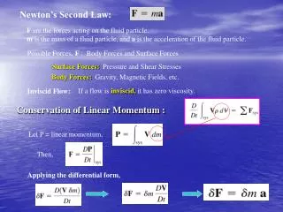
Newton’s Second Law: F are the forces acting on the fluid particle. m is the mass of a fluid particle, and a is the acceleration of the fluid particle. Possible Forces, F : Body Forces and Surface Forces Surface Forces: Pressure and Shear Stresses Body Forces: Gravity, Magnetic Fields, etc. If a flow is inviscid, it has zero viscosity. Inviscid Flow: Conservation of Linear Momentum : Let P = linear momentum, Then, Applying the differential form,

Surface Forces: Body Forces: Normal Stress: Shear Stress: Then the total forces:

Looking at the various sides of the differential element, the shear and normal stresses are shown for an x-face.

In components: For x-component, Divide by Material derivative for a Force Terms (1)

Viscosity effects for a Newtonian Fluid Shear Stresses: Normal Stresses: 식(1)에 대입 Navier-Stokes Eqn (x –direction)

Viscous Flows: Navier-Stokes Equations French Mathematician, L. M. H. Navier (1758-1836) and English Mathematician Sir G. G. Stokes (1819-1903) formulated the Navier-Stokes Equations by including viscous effects in the equations of motion. Sir G. G. Stokes (1819-1903) L. M. H. Navier (1758-1836) Terms in the x-direction: Weight term Pressure term Advective Acceleration (non-linear terms) Local Acceleration Viscous terms

Inviscid Flow : An inviscid flow is a flow in which viscosity effects or shearing effects become negligible. The equations of motion for this type of flow then becomes the following: Euler’s Equations ; In vector notation Euler’s Equation:

Inviscid Flow: Euler’s Equations Leonhard Euler (1707 – 1783) Famous Swiss mathematician who pioneered work on the relationship between pressure and flow. There is no general method of solving these equations for an analytical solution. The Euler’s equation, for special situations can lead to some useful information about inviscid flow fields.

Inviscid Flow: Bernoulli Equation From the Euler Equation, First, assume steady state: Select, the vertical direction as “up”, opposite gravity: Use the vector identity: Now, rewriting the Euler Equation: Rearrange:

Now, take the dot product with the differential length ds along a streamline: , is perpendicular to V, and thus to ds. ds and V are parrallel, We note, Now, combining the terms: Integrate: p d[ ] 1) Inviscid flow 2) Steady flow 3) Incompressible flow 4) Along a streamline Then,

Bernoulli’s Equation: Daniel Bernoulli (1700-1782) Swiss mathematician, son of Johann Bernoulli, who showed that as the velocity of a fluid increases, the pressure decreases, a statement known as the Bernoulli principle. He won the annual prize of the French Academy ten times for work on vibrating strings, ocean tides, and the kinetic theory of gases. For one of these victories, he was ejected from his jealous father's house, as his father had also submitted an entry for the prize. His kinetic theory proposed that the properties of a gas could be explained by the motions of its particles.

Bernoulli Equation : = H (total head) = constant Pressure Head 압력수두 Velocity Head 속도수두 Potential Head 위치수두 * 각항의 차원은 [L] 을 연결한 선= 에너지구배선(energy grade line) p. 212 그림4-18 을 연결한 선= 수력구배선(hydraulic grade line) =Total pressure = constant • 각항의 차원은 압력[F/L2] • 혹은 단위체적당 일(work)[F·L/L3] Hydrostatic Pressure 위치압력 Velocity (Dynamic) Pressure 동압 Static Pressure 정압

= Em =Total energy(단위 질량당 에너지) = constant Static energy Potential energy Kinetic energy Modified Bernoulli Equation : 마찰력이 있는 real fluid (수두손실:head loss) (압력손실:pressure loss) (에너지손실:energy loss)

Application of Bernoulli Equation: Free Jets Bernoulli Equation for along a streamline between any two points: Free Jets: Following the streamline between (1) and (2): 0 0 0 gage 0 gage h (대기압) (대기압) Torricelli’s Equation (1643년): Cv=coefficient of velocity Velocity at (5): Q(체적유량)=AV

Flow Rate Measurement through Orifice Z1=Z2이므로 Flowrate Measurements in Pipes : A0 A2 A1 Using continuity equation: P2 P1 Orifice So, if we measure the pressure difference between (1) and (2) we have the flow rate. Venturi Then, Qactual= A·Vactual

Pitot-Tube: Flow velocity (3) (3) Total Pressure = Static Pressure + Dynamic(velocity) Pressure Note: p1=γh and 0 0, no elevation 0, no elevation H. De Pitot (1675-1771)

제4장 HomeWork #5 4-3 4-7 4-11 4-14 4-15 4-18

Newton’s Second Law: