Download
1 / 22
220 likes | 339 Views
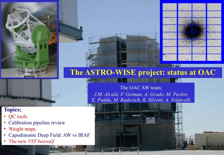
The ASTRO-WISE project: status at OAC. The OAC AW team: J.M. Alcalà, F. Getman, A. Grado, M. Pavlov, E. Puddu, M. Radovich, R. Silvotti, A. Volpicelli. Topics: QC tools Calibration pipeline review Weight maps Capodimonte Deep Field: AW vs IRAF The new VST beowulf. QC status (1).

E N D
The ASTRO-WISE project: status at OAC The OAC AW team: J.M. Alcalà, F. Getman, A. Grado, M. Pavlov, E. Puddu, M. Radovich, R. Silvotti, A. Volpicelli • Topics: • QC tools • Calibration pipeline review • Weight maps • Capodimonte Deep Field: AW vs IRAF • The new VST beowulf
QC status (3)
OAC QC tools 1) Sign test: correlated noise detection in bias frames 2)QCdome and QCtwilight: measure the relative flatness of dome and twilight flat fields 3) Outlayers: count the number of outlayers 4)Histo: check statistics (create histograms and compare with Gaussian distribution)
1)Sign test: correlated noise detection in bias frames the input frame is splitted in a number n of windows for each window, the excess of elements greater (or smaller) than the median of the whole frame is counted if this number is not compatible with the binomial distribution, the window is flagged the number of bad windows is compared with the number expected from the Gaussian distribution at a fixed number of sigmas and the quality index is obtained by: QI=(n_bad n_expected) /
2)QCdome and QCtwilight: measure the relative flatness of dome and twilight flat fields the input frame is normalised (divided by its median value) it is splitted in a number n of windows the median of each window is calculated the relative flatness is given by the diffe- rence between highest and lowest median forthe twilight FFs a cubic spline fit is used instead of the input image Test of QCdome on WFI frames. Left: V-band dome flats divided by their master. Right: same V-band dome flats divided by the B-band master.
Fig. 1 Fig. 2 Test of QCtwilight on WFI frames. Fig. 1: V-band dome flats divided by their master (left points) and by the B-band master (right points). Fig. 2: B-band dome flats divided by their master (left points) and by the V-band master (right points).
4)Histo: check statistics (create histograms and compare withGaussian distribution) The histo tool applied to a dome flat frame; note that the left panel is in logarithmic scale.
Calibration pipeline review: Overscan Correction Present algorithm (6 different methods): no overscan correction (default) median (prescan_x) median (overscan_x) median (prescan_y) median (overscan_y) average_per_row (prescan_x) currently used average_per_row (overscan_x)
Done !(07/11/03) Calibration pipeline review: Dome Flat Previous algorithm: normalise_by_mean (stack_by_median (normalise_by_mean (overscan_corrected (raw_dome) - master_bias ))) 1. overscan correction for each ‘raw_dome’ 2. master_bias subtraction 3. normalisation to 1.0 of each image by mean value 4. stacking by median 5. normalisation again We proposed: 1. overscan correction for each ‘raw_dome’ 2. master_bias subtraction 3. sigma_clip_average (including internal normalisation) 4. final normalisation
Done !(07/11/03) Calibration pipeline review: Twilight Flat Previous algorithm: normalise_by_mean (stack_by_median (normalise_by_mean (overscan_corrected (raw_twilight) - master_bias ))) 1. overscan correction for each ‘raw_twilight’ 2. master_bias subtraction 3. normalisation to 1.0 of each image by mean value 4. stacking by median 5. normalisation again We proposed: 1. overscan correction for each ‘raw_twilight’ 2. master_bias subtraction 3. sigma_clip_average (including internal normalisation) 4. final normalisation Note that in this case the sigma_clipping technique is even more important in order to remove stars from the raw twilight FFs !
Calibration pipeline review: Master Flat Present algorithm: normalise_by_mean ((M_dome / low_freq_component (M_dome)) low_freq_component (M_twilight)) 1. FFT of ‘master_dome’ 2. FFT of ‘master twilight’ 3. divide master dome by its low freq. component 4. multiply by low freq. component of master twilight 5. normalise to 1.0 by mean value Warning: The presence of bad pixels may introduce artificial frequencies that would be cut by FFT introducing errors. This problem can be critical for WFI data (e.g. CCD#3) other possible solutions: a)smoothing by running window (which can eventually have variable dimensions i.e. smaller windows near the edges) b) cubic spline interpolation
Calibration pipeline review: Fringing Pattern Present algorithm: norm_by_mean (stack_by_median (norm_by_median ((overscan_corrected (raw_science) - master_bias)/master_flat))) - 1.0 1. overscan correction for each ‘raw_science’ 2. master_bias subtraction 3. Master_FF correction 4. normalisation to 1.0 of each image by median value 5. stacking by median 6. normalisation again to 1.0 by mean value Note thatthis algorithmcontains already the assumption that the amplitude (or scaling factor) of the fringing is proportional to the background ! Otherwise we could not make any stacking. We suggest: To introduce the sigma_clip (with possible modifications) To divide each single corrected scientific frame by its low freq. component before combining them to obtain the fringing pattern, in order to obtain a uniform fringing amplitude across the field. The fringing pattern will then be multiplied by the low frequency component of each scientific frame before being subtracted to that scientific frame.
Calibration pipeline review: Reduced science frame Present algorithm: ((overscan_corrected (raw_science) master_bias) / master_flat) scaling_factor fringing_pattern Where scaling_factor is calculated with two different methods: a) minimisation of i,j(corrected_science scaling_factor fringing_pattern)2 ; high pixels (stars) are previously removed by a simple sigmaclip rejection b) scaling_factor is proportional to (background stars), where stars are removed using a simple sigmaclip of high pixels. Comments - suggestions: in the first method the present 20 sigma clipping is dangerous in crowded fields where the high presence of objects can lead to a bad solution ! The two scaling factors might be compared each other as a further QC test and saved in the DB for future trend analysis.
Calibration pipeline review: fringing scaling factor WFI scientific frame at 914 nm (CCD#1) corrected for bias and FF before and after fringing correction
Calibration pipeline review: fringing scaling factor Residual fringing: the same scientific frame is corrected for fringing using method a) and method b) to calculate the scaling factor.The difference shows aresidual amplitude of the order of 0.3 of the background (or 6 of the original fringing amplitude).
Calibration pipeline review: Performance INGESTION of 1 WFI extension: ~1 min for VST/OmegaCAM it would take half a day to ingest 100 Giga of raw data ! Total time to produce all the calibration frames~20 min (WFI frames); most of this time (~15 min) is used to create the Master Flat with FFTs. Fringing pattern scaling factors: computing times are ~150s and ~10s respectively using the two methods described in the previous slide. By the way, the 150s can be easily reduced improving the algorithm (derivative=0 instead of 30 iterations cycle), as already suggested by Mike Pavlov. FFTs are quite heavy in terms of computing time; using smoothing or cubic spline interpolation instead of FFTs would reduce the times needed to produce calibration frames from ~20 to less than 10 minutes
Pixel and weight maps Current scheme: weight_map=flat (hot_map cold_map cosmic_map) We propose: to flag also high pixels (close to the saturation) in raw scientific frames to compute more realistic weight maps, considering all the errors introduced by each step of the reduction (overscan, bias, FF, fringing): weight_map=(1/D)1/2 (hot_map cold_map saturated_map cosmic_map) where: D(i,j) sigma2 (i,j) = D[bias_corrected](i,j) D[master_flat](i,j) / master_flat(i,j)4 + D[master_flat](i,j) bias_corrected_frame(i,j)2 / master_flat(i,j)4 + D[bias_corrected](i,j) / master_flat(i,j)2
Calibration pipeline review: a few more comments To use average instead of median reduces errors: D[median]/D[average] = Pi/2 1.57 It can happen that fringing is present also on the dome flats (in WFI data we see sometime this effect, due to the sky light entering the dome). With the present algorithm for the master flat this is critical because fringing is not removed from dome flats (whereas it is removed from twilight flats).
Capodimonte Deep Field: AW vs IRAF The comparisons will consider two broad band filters (V and R) + one medium band at 914 nm (where the fringing is maximum). As a first step we plan to compare: 1.Master FF 2. Flatness of the reduced images. 3. Residual fringing. 4. Instrumental magnitudes of the point sources (obtained running Sextractor, with same parameters, on single exposures) in the different CCDs and in the different parts of each CCD. 5. Zero points and color terms from the standard fields.
The new VST beowulf Master: MB: Tyan 2880 CPU: two Opteron 244 RAM: 6 GB DDR PC2700 ECC registered DISK: 40 GB system Case: rack mount 2U Storage: 1.5 TB disks + 3 ware 7506 16 Nodes: MB Tyan 2880 CPU: two Opteron 244 RAM: 2 GB DDR PC2700 ECC registered DISK: 40 GB system Case: rack mount 2U Switch:24 ports Gigabit KVM:18 ports