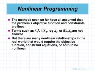
Nonlinear Programming
Nonlinear Programming. McCarl and Spreen Chapter 12. Optimality Conditions. Unconstrained optimization – multivariate calculus problem. For Y=f(X), the optimum occurs at the point where f '(X) =0 and f’''(X) meets second order conditions


Nonlinear Programming
E N D
Presentation Transcript
Nonlinear Programming McCarl and Spreen Chapter 12
Optimality Conditions • Unconstrained optimization – multivariate calculus problem. For Y=f(X), the optimum occurs at the point where f '(X) =0 and f’''(X) meets second order conditions • A relative minimum occurs where f '(X) =0 and f’''(X) >0 • A relative maximum occurs where f '(X) =0 and f’''(X) <0
Concavity and Second Derivative local max and global max local max f’’(x)<0 f’’(x)>0 f’’(x)<0 f‘’(x)>0 local min local min and global min
Multivariate Case • To find an optimum point, set the first partial derivatives (all of them) to zero. • At the optimum point, evaluate the matrix of second partial derivatives (Hessian matrix) to see if it is positive definite (minimum) or negative definite (maximum). • Check characteristic roots or apply determinental test to principal minors.
Determinental Test for a Maximum – Negative Definite Hessian f11 f12 f13 f21 f22 f23 f31 f32 f33 < 0 These would all be positive for a minimum. (matrix positive definite) f11 f12 f21 f22 > 0 < 0 f11
Global Optimum A univariate function with a negative second derivative everywhere guarantees a global maximum at the point (if there is one) where f’(X)=0. These functions are called “concave down” or sometimes just “concave.” A univariate function with a positive second derivative everywhere guarantees a global minimum (if there is one) at the point where f’(X)=0. These functions are called “concave up” or sometimes “convex.”
Multivariate Global Optimum If the Hessian matrix is positive definite (or negative definite) for all values of the variables, then any optimum point found will be a global minimum (maximum).
Constrained Optimization • Equality constraints – often solvable by calculus • Inequality constraints – sometimes solvable by numerical methods
Equality Constraints Maximize f(X) s.t. gi(X) = bi Set up the Lagrangian function: L(X,) = f(X) - ii(gi(X)-bi)
Optimizing the Lagrangian Differentiate the Lagrangian function with respect to X and . Set the partial derivatives equal to zero and solve the simultaneous equation system. Examine the bordered Hessian for concavity conditions. The "border" of this Hessian is comprised of the first partial derivatives of the constraint function, with respect to , X1, and X2.
Bordered Hessian Note: the determinant is designated |H2| For a max, the determinant of this matrix would be positive. For a min, it would be negative. For problems with 3 or more variables, the “even” determinants are positive for max, and “odd” ones are negative. For a min, all are negative.
Aside on Bordered Hessians You can also set these up so that the border carries negative signs. And you can set these up so that the border runs along the bottom and the right edge, with either positive or negative signs. Be sure that the concavity condition tests match the way you set up the bordered Hessian.
Example Minimize X12 + X22 s.t. X1 + X2 = 10 L = X12 + X22 - (X1 + X2 – 10) L/X1 = 2X1 - = 0 L/X2 = 2X2 - = 0 L/ = -(X1 + X2 -10) =0
Solving From first two equations: X1* = X2* = */2 Plugging into the third equation yields: X1*=X2*=5 and * = 10
Second Order Conditions For this problem to be a min, the determinant of the bordered Hessian above must be negative, which it is. (It’s -4)
Multi-constraint Case 3 constraints – g, h, and k 3 variables – 1, 2, 3
Multiple Constraints SOC M is the number of constraints in a given problem. N the number of variables in a given problem. The bordered Principle Minor that contains f22 as the last element is denoted |H2| as before. If f33 is the last element, we denote |H3|, and so on. Evaluate |Hm+1| through |Hn|. For a maximum, they alternate in sign. For a min, they all take the sign (-1)M
Additional Qualifications Examine the Jacobian developed from the constraints to see if it is full rank. If it is not full rank, some problems may arise. (The Jacobian is a matrix of first partial derivatives.)
Interpreting the Lagrangian Multipliers The values of the Lagrangian multipliers (i) are similar to the shadow prices from LP, except they are true derivatives (i = L/bi) and are not usually constant over a range.
Inequality Constraints Maximize f(X) s.t. g(X) b X 0
Example Minimize C = (X1 – 4)2 + (X2 –4)2 s.t. 2x1 + 3x2 ge 6 -3x1 – 2x2 ge –12 x1, x2 ge 0
Graph Optimum: 2 2/13, 2 10/13
A Nonlinear Restriction Maximize Profit = 2x1 + x2 s.t. -x12 + 4x1 - x2 le 0 2x1 + 3x2 le 12 x1, x2 ge 0
Graph – Profit Max Problem F1 F2 There is a local optimum at edge of F1, but it isn't global.
The Kuhn-Tucker Conditions • xf(X*) - * xg(X*) 0 • [ xF(X*) - * xg(X*)]X* = 0 • X* 0 • g(X*) b • *(g(X*)-b) =0 • * 0 represents the gradient vector (1st derivatives)
Economic Interpretation fj is the marginal profit of jth resource. i is shadow price of ith resource gij is the amount of the ith resource used to produce the marginal unit of product j. The sum-product of the shadow prices of the resources and the amounts used to produce the marginal unit of product j is the imputed marginal cost. Because of complementary slackness if j is produced, the marginal profit must be equal to imputed marginal cost.
Quadratic Programming Objective function is quadratic and restrictions are linear. These problems are tractable because the Kuhn-Tucker conditions reduce to something close to a set of linear equations. Standard Representation: Maximize CX – 1/2X'QX s.t. AX b X 0 (Q is positive semi-def.)
Example Maximize 15X1 + 30X2 + 4X1X2 –2X12 – 4X22 s.t. X1 + 2X2 30 X1, X2 non-negative C= [15 30] Q = [ ] • -4 • -4 8 A = [ 1 2 ] b = 30
Kuhn-Tucker Conditions • 15 + 4X2 – 4X1 - 1 0 • X1(15 + 4X2 – 4X1 - 1 ) = 0 • 30 + 4X1 – 8X2 - 2 1 0 • X2(30 + 4X1 – 8X2 - 2 1 ) = 0 • X1 + 2X2 – 30 0 • 1(X1 + 2X2 – 30) = 0 • X1, X2, 1 0
Reworking Conditions • -4X1 + 4X2 - 1 + s1 = -15 • 4X1 - 8X2 - 2 1 + s2 = -30 • X1 + 2X2 + v1 = 0 Now condition 2 can be expressed as X1s1=0 and condition 4 can be expressed as X2s2 =0 and condition 5 becomes 1v1=0. We can make one constraint X1s1 + X2s2 + 1v1=0
A Convenient Form • 4X1 - 4X2 + 1 - s1 = 15 • - 4X1 + 8X2 + 2 1 -s2 = 30 • X1 + 2X2 + v1 = 0 • X1s1 + X2s2 + 1v1=0
Modified Simplex Method A modified simplex method can be used to solve the transformed problem. The modification involves the "restricted-entry rule." When choosing an entering basic variable, exclude from consideration any nonbasic variables whose complementary variable is already basic.
Example Maximize 10X1 + 20X2 + 5X1X2 –3X12 – 2X22 s.t. X1 + 2X2 10 X1 ≤ 7 X1, X2 non-negative
Kuhn-Tucker Conditions • Derive the Kuhn-Tucker conditions for this problem. • L = Z (X1, X2) + i gi (X1, X2) • L / X1 <= 0 L / X2 <= 0 • X1 (L / X1) = 0 X2 (L / X2) = 0 There are two constraints in this problem.
Kuhn-Tucker The Kuhn-Tucker condition for the above problem; F.O.C. with respect to X1 and X2: 10 –6 X1+5X2 - 1 - 2 <= 0 (these 1 and 2 come from two inequalities) X1 (10 –6 X1 + 5X2 - 1 - 2 ) = 0 20 - 4X2 + 5X1 - 21 <= 0 X2 (20 –4X2 + 5X1 - 21 ) = 0 From the constraint inequalities; X1 + 2X2 <= 10 or 1 (X1 + 2X2 - 10) =0 X1 <= 7 or 2 (X1- 7) = 0 X1, X2, 1, 2 >= 0