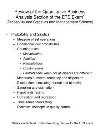
Review of the Quantitative Business Analysis Section of the ETS Exam * (Probability and Statistics and Management Scienc

1. Review of the Quantitative BusinessAnalysis Section of the ETS Exam*(Probability and Statistics and Management Science) • Probability and Saistics • Measure of set operations • Conditional/joint probabilities • Counting rules • Multiplication • Addition • Permutations • Combinations • Permutations when not all objects are different • Measures of central tendency and dispersion • Distributions (including normal and binomial) • Sampling and estimation • Hypothesis testing • Correlation and regression • Time-series forecasting • Statistical concepts in quality control *Slides available at H:\ditri\Teaching\Review for the ETS exam

2. Review of the Quantitative BusinessAnalysis Section of the ETS Exam • Management science • Linear programming • Project scheduling (including PERT and CPM) • Inventory and production planning • Special topics • queuing theory • simulation, and • decision analysis

3. Probability and Statistics • Measure of set operations • “Set” is a collection of objects • Sets are defined by the elements in the set (usually numbers) • Sets are usually labeled with letters and there will be a universal set (U) containing all elements in question • In statistics we are frequently interested in the set of real numbers from 0 to 1 • Usually interested in “subsets” that meet our requirements out of the universal set of 4 stems on an exam question we want the subset that contains the right answer • There can be a null set, that is one that does not meet all the requirements and is empty • Venn diagrams can be used to describe set operations

4. Venn Diagrams A union B A intersection B A complement

5. Conditional/Joint Probabilities • Probability • Real number from 0 to 1 mapping the likelihood of an “event” to the set of real numbers • An event is a set of possible outcomes • Events come in two flavors • Independent • Knowledge of one event does not provide insight into another event • Non independent events • Correlated events where knowledge of the outcome of one event changes the likelihood of another event • Conditional probabilities • Joint probabilities • Multidimensional situation where we are interested in more than one numeric characteristic

6. n1 n2 n2 n1 Counting Rules • Multiplication • (Decision tree) where subsequent outcomes depend on prior outcomes • N (total number of events) = n1 * n2 … nk where • ni is the number of events at each stage • Addition • Parallel activities • N = n1 + n2 + ….nk • Permutations (number of distinct orders) • Ordering n distinct items • An orange, apple, and a grapefruit • OAG, OGA, AOG, AGO, GAO, and GOA • With 0! = 1

7. Counting Rules(continued) • Permutations (continued) • Subset of r items from n distinct items • Number of distinct poker hands (including order dealt with each card regarded as unique) • Combinations • Distinct hands without regard to order • Or “n choose r” • Permutations when not all objects are different

8. Measures of Central Tendency and Dispersion • Random variables described by distributions • Captures the fact that more than one value per variable and some values are more common than others • Measures of central tendency • Mean • Mode (most frequent) • Median (“middle” value) • Measures of dispersion • Range (largest minus the smallest) • Standard deviation

9. Distributions(including normal and binomial) • As the name implies, we are describing how the frequency of various outcomes is distributed • Comes in two flavors • Probability distribution function • Measures the rate at which we accumulate probability (analogous to velocity) • Usually labeled f(x) • Cumulative distribution function • Measures the total accumulated probability (analogous to distance) • For discrete random variables • For continuous random variables

10. Normal Probability and Cumulative Distribution Functions

11. Binomial Distribution • Discrete, considering “yes” or “no” phenomena • Common in quality where products are “good” or “bad” • Usual case to have a sample of size n inspected and we are interested in the probability of seeing k (k = 0, 1, 2, …n) defects • Formally • Probability and Cumulative Distribution functions

12. Sampling and Estimation • Defined measures of central tendencies and dispersion earlier • Often, the parameters describing the population are not assessable • Might be too large to measure • Measuring process can be destructive • Measurement process itself might be biased (as is the case with how the census is compiled in your country) • Addressed by drawing a representative subset (a sample) and use inference to estimate the analogous parameters in the population • We can estimate mu and sigma in the population , using the X-bar and the standard deviation of the sample • X-bar and S are unbiased estimators of mu and sigma—that is, on average they accurately predict the estimated parameters

13. Hypothesis Testing • A testable idea • Based on the premise that science never knows, only rejects the null hypothesis at higher levels of statistical significance • My favorite example—our legal system • ‘People are presumed innocent until it is too unlikely (“beyond a reasonable doubt”) that the person is actually innocent • Upon rejecting the null, the person is sent to jail (there is always a chance the perp was indeed innocent) • Commonly used to test for differences in means (ANOVA) • Question: is the difference in sales levels for different cereal box designs the result of random chance or does one design sell better than another • H0: Sales levels are the same • HA: There is a difference in sales levels • Rejection of the null is based on the “p value” the probability of seeing a difference of the observed magnitude or more by chance

14. Correlation and Regression • Correlation • If random variables are not independent, we are interested in describing the relationship • Pearson Correlation Coefficient (r)

15. Y Distance Y = b0 + b1X1 Hole Deviation X Hours of Service Correlation and Regression • Regression • Captures the relationship between an independent and dependent variable • Goal is to achieve a “best fit” of a math model

16. Correlation and Regression • Regression • Objective is to explain variation in the data set • Coefficient of determination (R2) describes the proportion of variation explained by the model • In addition to R2, quality of model is assessed by • Significance of the model (measured with an F statistic) • Significance of estimated beta values (measured with t statistics) • Assurance the residuals exhibit “white noise” • Normally distributed • Mean zero • Constant variance • Independent

17. Time-series Forecasting • Two issues • Creating forecasts • Evaluating forecasts • Time-series methods • Average sets of data to make predictions of future events • Do not address causal issues—data sets “speak” for themselves • Issue is seeking a balance between “responsive” forecasting methods (respond to changes rapidly but are noisy) and filtering (averaging out of random fluctuations might be over damped) • Nomenclature: At = actual demand in period t Ft = forecast for period t n = number of observations in forecast t = number of the current period

18. Time-series Forecasting • Simple moving average • Weighted moving average • With • Exponential smoothing • Simple formula • with • Forecast is adjusted for the error • Masks a very sophisticated weighting scheme that considers all data points • Can be modified (Holt’s and Winter’s methods) to consider trends and seasonal effects

19. Time-series Forecasting • Wide assortment of forecasting methods (and possible parameters) • Wide assortment of evaluation methods • All look at averaging the errors • Bias is a simple average of the errors • Mean Absolute Deviation is an average of the absolute values of the errors • Standard Deviation and Mean Squared Error measures are averages of the squared errors • Mean Average Percentage Error is an average of the error scaled period by period • Two major groups • Absolute (average of errors) • Relative (average errors are scaled)

20. Bias Relative Forecast Error = AD* Major Evaluation Procedures Evaluation Method What is Done Absolute Version Relative Counter Part et = Ft-Dt Bias Mean Absolute Deviation MAD Mean Deviation = et = /Ft-Dt/ AD* SD Coefficient of Variation = Standard Deviation et = (Ft-Dt)2 AD* Mean Squared Error et = (Ft-Dt)2 Mean Average Percentage Error

21. Statistical Concepts in Quality Control • Been there, done that • Process control charts are nothing but the sampling distributions turned on their sides • Mean as the center and then upper and lower control limits drawn at three standard deviations (need to decide on the size of the sample) • Acceptance sampling is based on the binomial distribution discussed earlier • Again, decide on the sample size • Set “cutoff” values for the number of defects found in the sample

22. Process Control Charts Control Charts Illustrates when there is variation due to an assignable cause

23. Statistical Quality Control Models

24. Linear Programming

27. Project Scheduling(including PERT and CPM) • Some history • Both date from the 1950’s • CPM => DuPont • PERT => Polaris submarine project • Fundamentals • activities are unique branches (or nodes) • capturing • time and • precedence • additional precedence relationships can be modeled using dummy activities • CPM (critical path method) is deterministic • Project Evaluation and Review Technique is stochastic

28. Example Problem 2 7 B(5) • Issue is determining the critical path • Activities where the slack is zero • Activities that determine the expected completion time for the network 7 0 2 7 10 2 A(2) D(3) 0 7 10 2 2 6 C(4) 7 3

29. Converting Intuition into a Mean and Standard Deviation Most likely (modal) time (m) Expected time (te) Optimistic time (a) Pessimistic time (b)

30. Mean and Variance of theEntire Project • Based on summing the expected times and expected variability along the critical path • Assumptions: • Activity times are independent • There is one critical path • Project completion time is normally distributed • Te is the sum of the tes on the critical path • Where tei is the expected activity time for each of the N activities along the critical path.

31. Measure of the Variability in the Expected Completion Time for theEntire Project • Nature adds variability through the variance not the standard deviation Normal Distribution Te sTe

32. Inventory and Production Planning Forms of Inventory • Consider the transformation process: • Purchasing => • Operations => • Distribution • Raw materials (RM) • Work-in-Progress (WIP) • Finished Goods (FG) • Maintenance, Repair and Operating Expenses (MRO) • Manufacturing Inventory • RM + WIP + MRO

33. Classical Production Planning Hierarchy Business Plan Sales Plan Production Plan (aggregate production plan) Forecasts Master Production Scheduling Rough Cut Capacity Planning Material Requirements Planning Capacity Requirements Planning Shop Floor Control Purchasing (external factory)

34. Cycle Inventory Levels O n H a n d I n v e n t o r y i n U n i t s Time Between Orders(f) Demand Rate Q Q/2 = Average Cycle inventory Time

35. Types of Costs • Inventory holding rate • Time value of money • Insurance • Storage space • Risk • Obsolescence • Loss • Damage • Ordering Cost/Setup Cost • Stockout Costs • Backorder cost

36. Measuring Inventory Management Turnover = Annual Sales (at cost) Average Inventory Generally assumed that larger numbers are better, if . . . customer service stays high. Coverage = Average Inventory per period sales Weeks of Supply = Average Inventory (at cost) weekly sales Generally assumed that smaller numbers are better if . . . customer service stays high.

37. MRP - The System MPS Inventory Records BOM File MRP Planned Orders

38. A C B (2 req’d) C 3 4 5 1 2 6 Item A 18 8 42 15 12 5 Gross Req’ts Sched. Rec’ts On Hand 21 Planned Orders Order Q. = 20; Lead T. = 1; Safety S. = 0 3 4 5 1 2 6 Item B Gross Req’ts 32 Sched. Rec’ts On Hand 20 Planned Orders Order Q. = 40; Lead T. = 2; Safety S. = 0 3 4 5 1 2 6 Item C Gross Req’ts Sched. Rec’ts On Hand 50 Planned Orders Order Q. = LFL; Lead T. = 1; Safety S. = 10

39. Special TopicsQueuing Theory • Part of field of Stochastic Processes (those based on uncertainty) • Among others, Markov processes • Works from “states” where issue is probability of jumping to another brand • Seeks long term equilibrium state • “Birth Death” processes • Describe maintenance problems where • Machines “die” when they fail and are “reborn” when repaired • Interested in cost effective trade-off—customer’s time versus “servers”

40. The Queuing System • Arrivals—entities entering the system from a population (follows a statistical distribution—usually exponential) • Population • Finite, limited size or group of customers • Statistical properties change when someone enters the queuing system • Infinite size (usual case) • Queue discipline • Service rules (FIFO, LIFO, etc) • “Balking” • Number of servers • Line switching

41. Common Waiting Line Models

42. Special TopicsSimulation • A simulation is a computer-based model used to run experiments on a real system • Typically done on a computer • Determines reactions to different operating rules or change in structure • Can be used in conjunction with traditional statistical and management science techniques SimulationDefined

43. Major Phases in a Simulation Study Start Define Problem Construct Simulation Model Specify values of variables and parameters Run the simulation Evaluate results Validation Propose new experiment Stop

44. Data Collection & Random No. Interval Example Suppose you timed 20 athletes running the 100-yard dash and tallied the information into the four time intervals below You then count the tallies and make a frequency distribution Then convert the frequencies into percentages You then can add the frequencies into a cumulative distribution Finally, use the percentages to develop the random number intervals Seconds 0-5.99 6-6.99 7-7.99 8 or more Freq. 4 10 4 2 % 20 50 20 10 Accum. % 20 70 90 100 RN Intervals 00-19 20-69 70-89 90-99

45. Types of Simulation Models • Continuous • Based on mathematical equations • Used for simulating continuous values for all points in time • Example: The amount of time a person spends in a queue • Discrete • Used for simulating specific values or specific points • Example: Number of people in a queue

46. Desirable Features of Simulation Software • Be capable of being used interactively as well as allowing complete runs • Be user-friendly and easy to understand • Allow modules to be built and then connected • Allow users to write and incorporate their own routines • Have building blocks that contain built-in commands • Have macro capability, such as the ability to develop machining cells • Have material-flow capability • Output standard statistics such as cycle times, utilization, and wait times • Allow a variety of data analysis alternatives for both input and output data • Have animation capabilities to display graphically the product flow through the system • Permit interactive debugging

47. Advantages of Simulation • Often leads to a better understanding of the real system • Years of experience in the real system can be compressed into seconds or minutes • Simulation does not disrupt ongoing activities of the real system • Simulation is far more general than mathematical models • Simulation can be used as a game for training experience • Simulation provides a more realistic replication of a system than mathematical analysis • Simulation can be used to analyze transient conditions, whereas mathematical techniques usually cannot • Many standard packaged models, covering a wide range of topics, are available commercially • Simulation answers what-if questions

48. Disadvantages of Simulation • There is no guarantee that the model will, in fact, provide good answers • There is no way to prove reliability • Building a simulation model can take a great deal of time • Simulation may be less accurate than mathematical analysis because it is randomly based • A significant amount of computer time may be needed to run complex models • The technique of simulation still lacks a standardized approach

49. Overview of Decision Analysis • Definitions • i indexes decision alternatives • j indexes states of nature • Decision Alternative (Ai) • States of Nature (Sj) • Payoff (Vij) (intersection of Ai and Sj) • Regret (Rij) • Without information (game theory) • MaxiMax • MaxiMin • MiniMax regret • Decisions with uncertainty • Expected value of perfect information • Payoff tables (newsperson problem) • Decision trees

50. Decision Analysis-Decision Trees • A decision tree is a graphical representation of every possible sequence of decision and random outcomes (states of nature) that can occur within a given decision making problem. • A decision tree is composed of a collection of nodes (represented by circles and squares) interconnected by branches (represented by lines).