Business Statistics Autumn 2008
Business Statistics Autumn 2008 Chicago GSB C. Alan Bester About this Course Below is a link to the course website. Please visit and bookmark this site NOW. http://faculty.chicagogsb.edu/alan.bester/teaching/ Please review the syllabus and Course FAQ .

Business Statistics Autumn 2008
E N D
Presentation Transcript
Business StatisticsAutumn 2008 Chicago GSB C. Alan Bester
About this Course • Below is a link to the course website. Please visit and bookmark this site NOW. http://faculty.chicagogsb.edu/alan.bester/teaching/ • Please review the syllabus and Course FAQ. • Links to the data and many in class examples are embedded in these notes, and are also available by browsing the course website.
“Statistical Method” (We’ll start here) Formulate problem Get some data Visualize the data Do some statistical calculations Interpret results
Notes1: Data: Plots and Summaries 1. Data 2. Looking at a Single Variable 2.1 Tables 2.2 Histograms 2.3 Dotplots 2.4 Time Series Plots 3. Summarizing a Single Numeric Variable 3.1 The Mean and Median 3.2 The Variance and Standard Deviation 3.3 The Empirical Rule 3.4 Percentiles, quartiles, and the IQR 4. Looking at Two Variables 4.1 Categorical variables: the Two-way table 4.2 Numeric variables: Scatter Plots 4.3 Relating Numeric and Categorical variables
5. Summarizing Bivariate Relations 5.1 In Tables 5.2 Covariance and Correlation 6. Linearly related variables 6.1 Linear functions 6.2 Mean and variance of a linear function 6.3 Linear combinations 6.4 Mean and variance of a linear combination 7. Linear Regression 8. Pivot Tables (Optional) Note: As you’ve probably noticed, there are lot of slides. That is partly because I like to restate ideas and limit the number of concepts on any single slide. You will find there are really only a handful of “big ideas” that we will develop throughout the quarter…
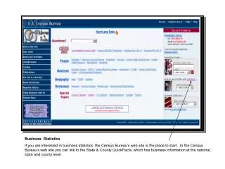
1.Data Here is some data (our sample): . . . (many more rows !!) The data is from a large survey carried out by a marketing research company in Britain. (Marketing data) Each row corresponds to a household. Each column corresponds to a different feature of the household. The features are called variables. The rows are called observations.
Most data sets come in this form. A rectangular array. Rows are observations. Columns are variables. Variables are the fundamental object in statistics. They come in several types.
The variable labeled "age" is simply the age (in years) of the responder. This is a numeric variable. This variable has units, and averages are interpretable. In contrast, the variable "Reg" is the geographical region of the household. Each "number" is really just a code for a region: A variable like Reg is called categorical. Think of: numeric vs. categorical quantitative vs. qualitative
Instead of using numbers we could have used text strings in the data file, that is, Reg: 3 3 2 1 . . Reg: North North North_West Scotland . . Instead of we could have But it is extremely common to use numeric codes. Another example: Which Democratic candidate do you support? 1= Hillary Clinton, 2= John Edwards, 3= Barack Obama, 4= Bill Richardson
The variable soc is categorical. It takes on codes 1-6, with meanings: This is an ordered categorical variable. You can't think of it as a numerical measure but A < B < ... < E. (“A” is actually the lowest social grade) Soc is ordered like age, but does not have units. It does not really make sense to compute the difference or to average two soc measurements. It does make sense to difference two ages.
That pretty much covers it. Variables are either numeric, categorical, or ordered categorical. Of course a numeric variable is always ordered. For numeric variables we also have: A variable is discrete if you can list its possible values. Otherwise it is called continuous.
For example, the amount of rainfall in the City of Chicago this month is usually thought of as being continuous. As a practical matter, any variable is discrete since we put it in the computer. What it comes down to is, if there are a lot of possible values, we think of it as continuous. (This is not really that important now; it will be later when we get to probability.) For example, you might think of age as continuous even though we measure it in years and can easily list its possible values. Number of children is more likely to be thought of as discrete.
Again, a good rule when working with a numeric variable is to keep in mind the units in which it is measured. For example age has units years. Percentages, which are numeric, don't have units. But there are always units somewhere. For example, if we look at the percentage of income a household spends on entertainment, we are looking at one quantity measured in units of currency divided by another.
Here are the definitions of all the variables in the survey data set: age: age in years sex: 1 means male, 2 means female soc: we saw this edu: education, terminal age of education Reg: we saw this.
inc: income Note: Both edu and inc could have been numeric, but are broken down into ranges. They are thus ordered categorical. This is extremely common; with income there are actually good reasons for doing this!
cola, restE, juice, cigs indicate use of a product category. 1 if you use it, 0 if you don't. This is called a dummy variable. 1 indicates something "happened", 0 if not. So, cigs=1 means you purchase cigarettes. restE means "restaurants in the evening". This is extremely common. Often in statistics we are interested in “does something happen?”. Another example is approval ratings ( 1=approve ). We will work with a lot of dummy variables this quarter.
A dummy variable can take on two values, 0 or 1. We use dummy variables to indicate something, 1 if that something “happened”, 0 if it did not. The rest of the variables in the marketing data represent tv shows. They are dummies: 1 if you watch, 0 if you don't. antiq: antiques roadshow news: bbc news enders: east enders friend: friends simp: simpsons foot: "football" (soccer)
Now we can see that there are three types of variables in the data set. (i) Demographics: age through income (ii) Product category usage, (iii) Media exposure (tv shows). What is the point? Why collect this data? We want to see how product usage relates to demographics. What kind of people drink colas? We want to see how the media relates to product usage so that we can select the appropriate media to advertise in. If friends viewers tend to drink colas, that might be a good place to advertise your cola.
Important Note: You can always take a numeric variable and make it an ordered categorical variable by using bins. For example, instead of treating age as a numeric variable it is common to break it into ranges. 0-20: a1 21-30:a2 31-40:a3 41-50:a4 51-60:a5 61-70:a6 >70: a7 for example:
The simplest case is a dummy variable: where x is numeric For example, you could define someone to be "old" if older than 40 and "young" otherwise. d=1 then means "old" and d=0 means "young".
2. Looking at a Single Variable The most interesting thing in statistics is understanding how variables relate to each other. "Friends watchers tend to drink colas". "Smokers tend to get cancer". But it is still very important to get of sense of what variables are like on their own. Note: We’ll use the term “distribution” informally to talk about what a variable looks like (what does a typical value look like, how spread out are its values, etc.) We will use the term more formally when we study probability.
2.1 Tables To look at a categorical variable we use a table: How to make this table We simply count how many of each category we have. Note: We have 1000 observations total, so the numbers in this table must add to 1000.
I like to graph the table. This table makes it easy to see how different social grades are represented. Numbers at the bottom are categories. The height of each bar equals the number of observations in that category.
2.2 Histograms We take a numeric variable, break it down into categories and then plot the table as on the previous slide. Remember, the height of each bar = # of observations or “frequency” in that category. 35-40 means (35,40] that is, <35 x <=40.
Time between arrivals at a bank, in minutes. (Bank data) A histogram with a "heavy right tail" is called skewed right. You can guess what skewed left is.
Source: Nicolas P. B. Bollen and Veronika K. Pool, “Do Hedge Fund Managers Misreport Returns? Evidence from the Pooled Distributions”; original data from Center for International Securities and Derivatives Markets, University of Massachusetts 0 Here’s a histogram of monthly hedge fund returns from 1994 to 2005. Notice anything interesting?
Aside: Histograms can be displayed in different ways… The observations here are starting players in the NFL (on offense). The numbers on the vertical axis correspond to rounds of the NFL draft, while the length of each blue bar is the percentage of starting players drafted at that position (forget the red bars). The plots on the right show only quarterbacks and fullbacks. (Source) Don’t worry, all of our histograms will be like the previous two slides. “Aside” or “Optional” on a slide means you are not responsible for the material on that slide on an exam!
2.3 Dotplots It can be a hassle choosing the bins for a numeric variable. For discrete variables and/or small data sets, we can just put a dot on the number line for each value. (Beer data) nbeerm: the number of beers male MBA students claim they can drink without getting drunk nbeerf: same for females
. : : : : . . : : : : . . : . : : :.: : : : . . +---------+---------+---------+---------+---------+-------nbeerm . .. . : : . +---------+---------+---------+---------+---------+-------nbeerf 0.0 4.0 8.0 12.0 16.0 20.0 We call a point like this an outlier. Generally the males claim they can drink more, their numbers are centered or located at larger values. Note: The dot plot is giving you the same kind of information as the histogram.
2.4 Time Series Plots The survey data is what we call cross-sectional. The households in our survey are a (hopefully representative) cross section of all British households at a particular point in time. In cross-sectional data, order doesn’t matter. We can sort our households by age, social, etc. and none of our results change as long as we keep each row intact. Other examples would be samples were every row corresponded to a firm, a plant, a machine... With a time series, each observation corresponds to a point in time.
Daily data on the Dow Jones index: (Dow data) . . . For time series data, the order of observations matters. (1-May-00 comes before 2-May-00, etc.) The easiest way to visualize time series data is often simply to plot the series in time order.
Time series plot of the close series. How to make this plot
We could have data at various frequencies: daily, monthly, quarterly, annual. The kinds of patterns you will uncover can be very different depending on the frequency of the data. A current hot topic of research at the GSB is "high frequency data".
Monthly US beer production. Do you see a pattern? Would we see this pattern if we looked at annual data?
Time series plot of monthly returns on a portfolio of Canadian assets: (Country Portfolio returns) On the vertical axis we have returns. On the horizontal axis we have “time”. Do you see a pattern?
Here is the histogram of the Canadian returns. Notes: (i) The histogram does not depend on the time order. (ii) The appearance of the histogram depends on the number of bins. Too many bins makes the histogram appear “spiky”.
Taken from David Greenlaw, Jan Hatzius, Anil Kashyap, and Hyun Shin, US Monetary Policy Forum Report No. 2, 2008 Be careful. What pattern do you see in this series? How about now?
From same paper as the previous slide. Time series plots are also used to compare patterns across different variables over time, and sometimes to see the impact of past events (be very careful there, too).
3. Summarizing a Single Numeric Variable We have looked at graphs. Suppose we are now interested in having numerical summaries of the data rather than graphical representations. Two important features of any numeric variable are: 1) What is a typical or average value? 2) How spread out or ‘variable’ are the values?
The mean and median capture a typical value. The variance/standard deviation capture the spread. For example we saw that the men tend to claim they can drink more. How can we summarize this? . : : : : . . : : : : . . : . : : :.: : : : . . +---------+---------+---------+---------+---------+-------nbeerm . .. . : : . +---------+---------+---------+---------+---------+-------nbeerf 0.0 4.0 8.0 12.0 16.0 20.0
Monthly returns on Canadian portfolio and Japanese portfolio. They seem to be centered roughly at the same place but Japan has more spread. How can we summarize this?
3.1 The Mean and Median We will need some notation. Suppose we have n observations on a numeric variable which we call "x". the last number, n is the number of numbers,or the “number of observations.” You may also hear it referred to as the “sample size.” the first number xi is the value of x associated with the ithobservation (row).
Here, x is just a name for the set of numbers, we could just as easily use y. In a real data set we would use a meaningful name like "age". x 5 2 8 6 2 n=5 Sometimes the order of the observations means something. In our return data the first observation corresponds to the first time period. In the survey data, the order did not matter.
The sample mean is justtheaverage of the numbers “x”: We often use the symbol to denote the mean of the numbers x. We call it “x bar”.
Here is a more compact way to write the same thing… Consider We use a shorthand for it (it is just notation): This is summation notation.
Using summation notation we have: The sample mean:
Graphical interpretation of the sample mean Here are the dot plots of the beer data for women and men. Which group claims to be able to drink more? Character Dotplot . . . . : : . +---------+---------+---------+---------+---------+-------nbeerf . : : : : . . : : : : . . : . : : : . : : : : . +---------+---------+---------+---------+---------+-------nbeerm 0.0 2.5 5.0 7.5 10.0 12.5 In some sense, the men claim to drink more. To summarize this we can compute the average value for each group (men and women). Note: I deleted the outlier, I do not believe him!.
“On average women claim they can drink 4.2 beers. Men claim they can drink 7.9 beers” Mean of nbeerf = 4.2222 Mean of nbeerm = 7.8625 How to calculate these means In the picture, I think of the mean as the “center” of the data. Character Dotplot . . . . : : . +---------+---------+---------+---------+---------+-------nbeerf . : : : : . . : : : : . . : . : : : . : : : : . +---------+---------+---------+---------+---------+-------nbeerm 0.0 2.5 5.0 7.5 10.0 12.5 4.2 7.86
Let us compare the means of the Canadian and Japanese returns. Mean of canada = 0.0090654 Mean of japan = 0.0023364 This is a big difference as a practical matter! (Average monthly return of .90% versus .23%) It was hard to see this difference in the histograms because the difference is small compared to the variation.
More on summation notation (take this as an aside) Let us look at summation in more detail. means that for each value of i, from 1 to n, we add to the sum the value indicated, in this case xi. add in this value for each i