Download
1 / 26
260 likes | 373 Views
NET 2: Empirical Research on Network Effects Gandal, N., "Hedonic Price Indices for Spreadsheets and an Empirical Test for Network Externalities," Rand Journal of Economics (25), 1994, 160-70.

E N D
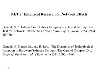
NET 2: Empirical Research on Network Effects Gandal, N., "Hedonic Price Indices for Spreadsheets and an Empirical Test for Network Externalities," Rand Journal of Economics (25), 1994, 160-70. Gandal, N., Kende, M., and R. Rob, “The Dynamics of Technological Adoption in Hardware/Software Systems: The Case of Compact Disc Players,” Rand Journal of Economics (31), 2000, 43-61.
Gandal, Rand Journal of Economics, 1994 Did spreadsheet programs that were compatible with Lotus command a premium? Idea is that compatibility gives users of your product access to other product’s network. Results not due to switching costs because the spreadsheet market was growing a lot b/w 1986 and 1991. Direct effects because people want to share files and indirect with compatible software e.g. database programs.
Paper uses product level data on spreadsheet prices and characteristics between 1986 and 1991 • Estimate hedonic pricing equations of form: • ln(pit) = Zit + it • Z are product attributes, one of which is a compatibility dummy, others “network” variables are dummies for linking capabilities between spreadsheets (LINKING), (GRAPHS). There is a variable that measures capacity of the spreadsheet as well. • By 1991, nearly all high end spreadsheets were compatible. That was not the case in 1986, when many of the premium brands were not compatible with Lotus format. • Article examines consumers’ valuation of compatibility, yet formally doesn’t address firms’ decisions to become compatible. Would need a structural model for this.
Data There is an unbalanced panel of 91 model-observations. In addition to the basic editing functions common to all spreadsheets, the DATAPRO report contains the following characteristics and features. I briefly summarize the available data. (1) The dummy variable LOCOMP takes on the value one if the program is compatible with the Lotus (WKS, WK1) format. Otherwise the variable takes on the value zero. If the program is compatible with the Lotus format, it is capable of exchanging files with Lotus and other spreadsheets that support the Lotus format. (2) The dummy variable RECALC takes on the value one (zero) if the program can (can not) automatically recalculate when new entries are made. (3) The dummy variable SORTING takes on the value one if the program can sort a group of data observations on at least two levels.
(4) The variable GRAPHS is a dummy variable that takes on the value one if the program is capable of performing all of the following basic graphs: pie, bar, and line. If the program cannot perform these basic functions, the variable GRAPHS takes on the value zero. These basic functions are bundled because the early DATAPRO reports collected the data in this manner. (5) The variable WINDOW takes on the value one if the maximum number of windows on-screen simultaneously is between two to fifteen and takes on the value two if this maximum is sixteen or more. If this feature is not available, the variable WINDOW takes on the value zero. This variable was defined in this manner because some spreadsheets offer a maximum that is limited only by hardware features. (6) The dummy variable LINKING takes on the value one if values in several worksheets can be updated at the same time.
(7) The dummy variable EXTDAT takes on the value one if the program provides links to external data bases, and zero otherwise. This link can be either proprietary or through SQL support. If this feature is available, databases on mainframes can be downloaded directly into the spreadsheet. (8) Macros allow a user to automate repetitive tasks. The dummy variable PROGRAM takes on the value one if macros can be written in this manner. (9) Macros can also be written in “learn mode.” In learn mode, the keystrokes that are to be replicated are typed and the spreadsheet converts these keystrokes into a Macro. The dummy variable LEARN takes on the value one if the program enables the users to automate repetitive tasks in this manner. (10) The dummy variable LANCOM takes on the value one if the program has the capability of linking independent users through a LAN.
(11) The dummy variable PRINT takes on the value one if three or more of the following five advanced print functions are possible: Sideways printing, Background Printing, Preview Mode, PostScript Support, and Printing of non-contiguous worksheet portions. (12) The variable PRESENT takes on the value one if worksheets and graphs can be printed on the same page OR if multiple printing fonts (and character sizes) are available. If both features are available, this variable takes on the value two, while if neither feature is available, the variable takes on the value zero. Although it seemed natural to group the two presentation features together, nothing in the analysis changes if these features are entered as separate variables. (13) The dummy variable LOTUS takes on the value one if the program is produced by Lotus Development Corporation and zero otherwise.
(14) The variable MINRC measures the power of the spreadsheet and is defined to be the minimum of the maximum number of rows and columns that the spreadsheet can handle. (15) The variable PRICE is the list price for a single copy of the program. (16) The variable LPRICE is defined to be the natural log of the price. (17) The variable LMINRC is defined to be the natural log of MINRC. Variables (1) through (6) are considered to be basic spreadsheet features, while variables (7) through (12) are more advanced features. Some of these advanced features (EXTDAT, PRESENT, and PRINT) were not available until 1989.
In addition, to the above information, the year in which the observation was taken and the date of introduction are available. This allows the construction of time, age and vintage dummy variables, which are important for the analysis. The time dummy variables are denoted TIME87, TIME88, TIME89, TIME90, and TIME91. Similar to the personal computer (hardware) market, most products in this market were less than two years old. In this sample, fully 54 percent of the spreadsheets were new, 26 percent had been available for one year, 9 percent were two years old and 11 percent had been available for three or more years. Lotus was the dominant firm throughout the period. Other major spreadsheets include Microsoft (first with Multiplan and then with Excel), Computer Associates (various versions of SuperCalc), Paperback Software (VP-Planner), WordPerfect (PlanPerfect) and Borland (Quattro and Quattro Pro) in the latter part of the sample.
TABLE 2: REGRESSION RESULTS (DEPENDENT VARIABLE IS LPRICE) Regression (#1) Regression (#2) Regression (#3) Regression (#4) All independent Variables Significant Variables Preferred equation New Models Only coeff. (t-stat) coeff. (t-stat) coeff. (t-stat) coeff. (t-stat) VARIABLES CONSTANT 3.73 (10.92) 3.76 (12.31) 3.12 (9.50) 2.61 (4.91) TIME87 -0.076 (-0.45) -0.062 (-0.38) -0.07 (-0.43) -0.57 (-1.73) TIME88 -0.42 (-2.37) -0.44 (-2.67) -0.45 (-3.03) -0.94 (-2.91) TIME89 -0.64 (-3.50) -0.70 (-4.20) 0.92 (1.71) 1.63 (1.65) TIME90 -0.74 (-4.13) -0.79 (-4.90) 0.90 (1.67) 1.47 (1.51) TIME91 -0.82 (-4.48) -0.85 (-5.30) 0.85 (1.59) 1.54 (1.56) LMINRC 0.11 (1.31) 0.11 (1.59) 0.26 (3.24) 0.41 (3.42) LOTUS 0.59 (3.46) 0.56 (4.36) 0.46 (3.62) 0.44 (1.97) GRAPHS 0.45 (2.94) 0.46 (3.51) 0.52 (4.18) 0.36 (2.03) WINDOW 0.17 (2.16) 0.17 (2.14) 0.14 (1.92) 0.18 (1.71) LOCOMP 0.76 (5.30) 0.72 (5.28) 0.66 (5.17) 0.70 (3.02) EXTDAT 0.52 (3.10) 0.55 (4.05) 0.57 (3.93) 0.67 (3.16) LANCOM 0.25 (1.62) 0.21 (1.65) LINKING 0.18 (1.51) 0.21 (1.91) 0.26 (2.00) 0.43 (2.22) LEARN 0.03 (0.18) PROGRAM 0.13 (0.70) PRESENT -0.08 (-0.54) PRINT 0.20 (0.86) SORTING -0.21 (-1.27) TLANCOM 0.61 (3.28) 0.33 (1.20) TLMINRC -0.34 (-3.07) -0.52 (-2.76) TLINKING -0.31 (-1.49) -0.25 (-0.76) No. Observations 91 91 91 49 S.E. of Regression .391 .385 .356 .385 R2 . 862 .857 .881 .875 ADJ. R2 . 827 .833 .857 .819
Price Indexes Table 3 shows the quality-adjusted (hedonic) price indexes for regressions 2,3 and 4 from Table 2. The numbers in parentheses are the percentage price declines from the previous year. The average yearly decline in quality adjusted prices was 15 percent for the full sample and 22 percent for new products in the sample. For the second regression, price indexes are calculated by taking the exponentiated estimated coefficients on the time dummy variables, with the coefficient on T86 normalized to zero. For regressions 3 and 4, the procedure is slightly more complicated. See Berndt and Griliches (1993) for details. Table 3. Price Indexes for Spreadsheets (1986=1.00) Year 1986 1987 1988 1989 1990 1991 Regression (#2 1.00 .94 (6.0) .64 (31.7) .49 (22.6) .45 (8.6) .42 (5.5) Regression (#3) 1.00 .93 (7.0) .64 (30.9) .50 (21.9) .48 (4.0) .46 (4.2) Regression (#4) 1.00 .57(43.0) .39 (31.6) .31 (20.5) .27 (12.9) .28 (-3.7) Percentage decline from previous year in parentheses
Further Tests of the Significance of Lotus Compatibility In the first subsample, 15 of the 40 model observations (38 percent) were not compatible with the Lotus platform and some of these "incompatible" spreadsheets were relatively expensive. This is not the case with the second subsample, in which 42 of the 51 model observations (82 percent) were compatible with the Lotus platform. Further, the spreadsheets not compatible with the Lotus platform in the second subsample ranged in price from $39.00 to $60.00, while the spreadsheets that were compatible with the Lotus platform ranged in price from $60.00 to $695.00. It is thus encouraging that the variable TLOCOMP (which is LOCOMP interacted with a dummy variable for the second (1989-1991) sample period) is insignificant in both regressions 3 and 4. Adding the variable TLOCOMP to regression 3, one obtains a coefficient (t-stat) of -0.12 (-0.53), while adding the same variable to regression 4 yields a coefficient (t-stat) of 0.02 (0.055). Thus, the Lotus compatibility parameter is essentially the same for both subsamples. Despite the fact that some of the incompatible spreadsheets were relatively expensive in the (1986-1988) subsample, the average price of a lotus compatible spreadsheet in this subsample ($365.00) is much higher than the average price of an incompatible spreadsheet ($80.00). Thus this subsample was further restricted to spreadsheets that cost less than $200.00. In this restricted sample of non-premium spreadsheets, there were 24 observations, of which 9 were compatible with the Lotus platform. The mean price of lotus compatible spreadsheets in this subsample was $151.00 versus $80.00 for the 15 incompatible spreadsheets. Gandal (1992) shows that although the lotus compatibility effect declines slightly in magnitude, it is still highly significant. Thus, the effect of Lotus compatibility continues to hold for non-premium spreadsheets.
Comments: • Common critique of all hedonic price equations is question of demand or supply effects (they are very reduced form). Is this really a premium or does it just cost more to make Lotus compatible spreadsheets? • Finds 93% premium for Lotus compatibility. (e.66 -1) • At first glance, the premium seems quite large, but once one thinks about the importance of compatibility… • Results are robust to all sectors of the market (premium, generics, etc.) • Gandal (1995) extends the results to Database Management Software and multiple standards. He finds similar results, but the only “important” standard is the Lotus (WK) standard.
Gandal, Kende, Rob (Rand Journal of Economics, 2000) The dynamics of technological adoption in hardware/software systems: the case of compact disc players First Structural Model used in Empirical Network Literature. See also Rysman (2001). This paper examines the diffusion of ahardware/software system. For such systems there is interdependence betweenthe hardware-adoption decisions of consumers and the supply decisions ofsoftware manufacturers. Paper considers the CD-industry and estimates the (direct) elasticityof adoption with respect to CD-player prices and (the cross) elasticity withrespect to the variety of CD-titles. Results show that the crosselasticity is significant. Model can be used to quantify the effect ofvarious policies aimed at speeding up the diffusion of a system.
Methodology useful for public-policy analysis regarding the benefits of backward compatibility for other systems. (Example HDTV). Firm strategy: it is claimed that high-tech firms can enhance their profits by subsidizing the adoption of their technology. (Elasticities of hardware sales with respect to hardware prices and with respect to software availability.) Dynamic model for estimating demand (technology adoption) is applicable even when there is no complementary software industry. Consumers explicitly trade-off the lower prices which will result from waiting one period with the loss of one period's services from the durable product.
Step 1: Learn about the CD industry. (Helpful for modeling purposes) Step 2: Informal reduced form regressions -- get feel for data Step 3: Develop a structural model. Step 4: Econometric Specification and Estimation of Structural Model. Step 5: Discuss, Interpret, and Check Robustness of the Results Step 6: Perform counterfactuals
Step 1: Key institutional details: (i) in the case of CD-players, hardware prices are essentially exogenous. Philips licensed the technology to more than 30 firms. Hardware market for compact disc players quite competitive. (ii) There are cost instruments for CD-variety. These cost instruments are the fixed cost of installing capacity for pressing compact discs. (iii) Record companies were integrated into the production of compact discs. The first CD (disc) pressing plant in the U.S was opened by Sony/CBS Records (of Japan) in 1984. The second plant was opened by Phillips/Polygram Records. CD production/recording industry was an integrated “software” industry
Step 3: Structural Model Entry decision of software firms: If a software firm enters at time t, lifetime profits are -Ft + t+1 + 2t+2 +… , where t+1 are operating profits from sales of software in period t+1. If a software firm waits and enters at time t+1, lifetime profits (calculated at time t) are -Ft+1 + 2t+2 +… (Enters at time t+1) Free entry equilibrium condition requires that benefit of waiting (cost savings) equal benefit from early entry Ft -Ft+1 = t+1 = Ytf(nt), where n = #of software firms, Y=installed base. (1) log f(nt) = -log - log Yt + log (Ft -Ft+1)
Consumer Adoption Decision is an individual characteristic measuring intensity of preference for the system, 0<< . The c.d.f. of is F(). The total number of potential buyers is M=F() If consumer purchases in period t, net benefit is: -Pt + [CS(pt+1) + 2CS(pt+2) +…], where P=hardware price, p=software price, CS=Consumer Surplus. If consumer purchases in period T+1, net benefit (evaluated at t) is: - Pt+1 + [2CS(pt+2) + 3CS(pt+3) +…]. Pt - Pt+1 = tCS(pt+1) = tg(nt). (Indifferent consumer) (2) log(t)=log(Pt - Pt+1) - log - log g(nt). _ _
4. Econometric Specification & Estimation F()=1 g(n)=anr f(n)=bn Comment: First assumption is somewhat different from what is usually done. People typically assume a bell-shaped distribution over . However, the assumptions give us tractable functional forms to estimate and the insight of the model -- that one should use cumulative variables -- is not dependent on these functional forms. (1*) log (Nt) = 0 + 1 log Yt + 2 log (Ft -Ft+1) + t , (2*) log (M-Yt)= b0 + b1 log (Pt -Pt+1) + b2 log Nt+ nt , where N=mn (m number of titles per firm); model implies 1 = -2 From the theoretical model, 1 >0, 2 <0, b1 >0, and b2 <0.
OLS Results with AR(1) terms are in Table 3 Instrumental Variables Estimation: Table 4 Cost Shifters (for Nt): log (Ft -Ft+1) , (Ft -Ft+1)2 Cost Shifters (for Yt): log (Pt -Pt+1) , (Pt -Pt+1)2 Theoretical direction of OLS bias: Estimates of cross coefficients biased away from zero; estimates of own coefficients biased towards zero. Results in Tables (3) and (4) consistent with theoretical direction of OLS bias.
5. Discussion/Interpretation of Results Elasticity of hardware sales with respect to variety of software: - b2(M-Yt)/Yt Elasticity of hardware demand with respect to a permanent percentage price cut: - b1(M-Yt)/Yt Ratio - b2/b1 is independent of time. From table (4), estimate of the ratio is 0.54. A 10 percent increase in CD titles would have had as large an effect on sales as a 5 percent price cut.
Robustness of the Results Potential Market (Index) M=300,000 (rather than 500,000). Both the price and variety effects nearly double in absolute value. But the estimate of the ratio (- b2/b1) remains essentially unchanged at 0.52. We also examined an alternative set of instruments. In the alternative case, we just employed log (Ft -Ft+1), as an instrument. In this case, the consumer adoption equation is exactly identified. The ratio (- b2/b1) remains essentially unchanged at 0.56. We also estimated the consumer adoption equation using first differences and estimated the consumer adoption equation using an alternative specification. See the paper for discussion.
6. Counterfactual: The Effect of Compatibility Assume that it had been possible to make CD-players compatible with LPs, and that the IV parameter estimates of table (4) describe the true diffusion process. Using simulations, we examine how compatibility could have accelerated the adoption process. We find that if the amount of variety had grown by 100 percent between the first and the second quarter of 1985 the diffusion process would have been shortened by 1.5 years. While this counterfactual is purely a ``thought experiment'' for the CD-system, it is of great relevance for other systems such as high-definition television (HDTV).