Decision Analysis
This comprehensive guide discusses the characteristics of good decision-making, focusing on logical reasoning, consideration of alternatives, and the application of quantitative analysis. It outlines the steps in decision analysis, including clearly defining problems and evaluating outcomes using expected monetary value (EMV). It further explores types of decision-making under certainty, uncertainty, and risk. Detailed examples illustrate concepts like expected value of perfect information (EVPI) and opportunity loss, alongside decision trees for complex decisions.

Decision Analysis
E N D
Presentation Transcript
Decision Analysis A. A. Elimam College of Business San Francisco State University
Characteristics of a Good Decision • Based on Logic • Considers all Possible Alternatives • Uses all Available Data • Applies Quantitative Approach Decision Analysis Frequently results in a favorable outcome
Decision Analysis (DA) Steps • Clearly define the problem • List all possible alternatives • Identify possible outcomes • Determine payoff for each alternative/outcome • Select one of the DA models • Apply model to make decision
Types of Decision Making (DM) • DM under Certainty: Select the alternative with the Maximum payoff • DM under Uncertainty: Know nothing about probability • DM under Risk: Only know the probability of occurrence of each outcome
Decision Table Example State of Nature (Market) Alternatives Favorable($) Unfavorable($) -180,000 Large Plant 200,000 -20,000 100,000 Small Plant Do Nothing 0 0
Decision Making Under Risk • Expected Monetary Value (EMV) EMV (Alternative i) = (Payoff of first State of Nature-SN) x (Prob. of first SN) +(Payoff of second SN) x (Prob. of Second SN) +(Payoff of third State of Nature-SN) x (Prob. of third SN) +. . . + (Payoff of last SN) x (Prob. of last SN)
Thompson Lumber Example • EMV(Large F.) = (0.50)($200,000)+(0.5)(-180,000)= $10,000 • EMV(Small F.) = (0.50)($100,000)+(0.5)(-20,000)= $40,000 • EMV(Do Nothing) = (0.50)($0)+(0.5)(0)= $0
Thompson Lumber State of Nature (Market) Alternatives Favorable ($) Unfavorable ($) EMV ($) Large Plant 200,000 -180,000 10,000 100,000 -20,000 Small Plant 40,000 0 0 Do Nothing Probabilities 0.5 0.5
Expected Value of Perfect Information (EVPI) • Expected Value with Perfect Information = (Best Outcome for first SN) x (Prob. of first SN) +(Best Outcome for second SN) x (Prob. of Second SN) + . . . + (Best Outcome for last SN) x (Prob. of last SN)
Expected Value of Perfect Information (EVPI) • EVPI = Expected Outcome with Perfect Information - Expected Outcome without Perfect Information • EVPI = Expected Value with Perfect Information - Maximum EMV
Thompson LumberExpected Value of Perfect Information • Best Outcome For Each SN • Favorable: Large plant, Payoff = $200,000 • Unfavorable: Do Nothing, Payoff = $0 • So Expected Value with Perfect Info. = (0.50)($200,000)+(0.5)(0)= $100,000 • The Max. EMV = $ 40,000 • EVPI = $100,000 - $40,000 = $ 60,000
Decision Table Example Possible Future Demand Alternative Low ($) High ($) 270 Small Facility 200 800 160 Large Facility Do Nothing 0 0
Example A.5 Demand Alternatives Low ($) High ($) EMV ($) 270 Small 200 242 160 800 Large 544 0 0 Do Nothing Probabilities 0.4 0.6
Example A.8Expected Value of Perfect Information • Best Outcome For Each SN • High Demand: Large , Payoff = $800 • Low Demand : Small , Payoff = $200 • So Expected Value with Perfect Info. = (0.60)($800)+(0.4)(200)= $560 • The Max. EMV = $ 544 • EVPI = $ 560 - $ 544 = $ 16
Opportunity Loss : Thompson Lumber State of Nature (Market) Favorable ($) Unfavorable($) 0-(-180,000) 200,000-200,000 0-(-20,000) 200,000-100,000 200,000-0 0 - 0
Opportunity Loss : Thompson Lumber State of Nature (Market) Alternatives Favorable ($) Unfavorable ($) EOL ($) Large Plant 0 180,000 90,000 100,000 20,000 Small Plant 60,000 Do Nothing 200,000 0 100,000 Probabilities 0.5 0.5
Sensitivity Analysis EMV, $ Point 2, p=0.62 EMV(LF) Point 1 p=0.167 200,000 EMV(SF) 100,000 EMV(DN) 0 1 -100,000 Values of P -200,000
Decision Trees • Decision Table: Only Columns-Rows • Columns: State of Nature • Rows: Alternatives- 1 DecisionONLY • For more than one Decision Trees • Decision Trees can handle a sequence of one or more decision(s)
Decision Trees • Two Types of Nodes • Selection Among Alternatives • State of Nature • Branches of the Decision Tree
Decision Tree: Example Favorable (0.5) Large Unfavorable (0.5) F. (0.5) Small U. (0.5) Do Nothing F. (0.5) U. (0.5)
A Decision Tree for Capacity Expansion(Payoff in thousands of dollars) Low demand [0.40] $70 Don’t expand $90 Small expansion High demand [0.60] ($109) 2 Expand 1 ($135) $135 Low demand [0.40] Large expansion ($148) $40 High demand [0.60] ($148) $220
Decision Tree for Retailer Low demand [0.4] $200 High demand [0.6] Small facility Don’t expand ($242) $223 2 Expand $270 ($270) 1 Do nothing $40 Modest response [0.3] 3 ($544) $20 Advertise Low demand [0.4] Large facility ($160) Sizable response [0.7] ($160) $220 High demand [0.6] ($544) $800