Download
1 / 43
460 likes | 683 Views
Radially Polarized Spherical Piezoelectric Acoustic Transducer. Introduction. This tutorial provides a step-by-step instruction to setup a 3D structural-acoustic interaction problem. Interaction between a vibrating piezoelectric structure with the surrounding fluid media is considered.

E N D
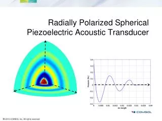
Radially Polarized Spherical Piezoelectric Acoustic Transducer
Introduction • This tutorial provides a step-by-step instruction to setup a 3D structural-acoustic interaction problem. • Interaction between a vibrating piezoelectric structure with the surrounding fluid media is considered. • Instructions on how to create a radially polarized piezoelectric material in spherical coordinates is provided. • The coupled multiphysics is solved as a stationary problem by considering frequency domain analysis.
Schematic of a spherical transducer Surrounding fluid Piezoelectric element Applied electric potential Ground
Start from the Model Navigator Acoustics Module > Piezo Solid > Frequency response analysis
Start from the Model Navigator Acoustics Module > Pressure Acoustics > Time-harmonic analysis
Set the excitation frequency Physics > Scalar variables We will use an excitation frequency of 25 kHz This will make the excitation frequency in acoustics (freq_acpr) and piezo solid (freq_smpz3d) to be the same
Number of waves we can capture We will use this information to create the modeling geometry such that we can capture two stationary waves in our model. Note that the larger the geometry, the higher the computation time and memory requirements.
Geometry – create a sphere Draw four spheres with the following radii: Sphere 1: r = 2.5e-3 Sphere 2: r = 3.5e-3 Sphere 3: r = 0.03 Sphere 4: r = 0.04 • The size of the 1st and 2nd spheres determines the thickness of the piezo element. • The size of the 2nd and 3rd spheres determines the thickness of the air domain. • The size of the 3rd and 4th spheres determines the thickness of the PML (perfectly matched layer).
Geometry Click on the Zoom Extents button to fit all the spheres on the GUI screen The outer PML layer approximates the solution at an infinite distance For modeling purpose, we will consider only 1/8th of the sphere by introducing symmetry planes. The solution for this model will hold good for this entire geometry or a part of it as long as the spherical symmetry is not violated.
2D work-plane Click on the Zoom Extents button to fit the projection of all the spheres on the xy-plane
The xy-plane of symmetry Create a square as shown above
Geometry with one embedded plane This is how the 3D geometry should look after embedding the square in the xy-plane We need to do the same for the yz and zx-planes.
Geometry with two embedded planes • Select the square in 3D geometry and copy-paste with zero displacements. • Go to Draw > Modify > Rotate. Use the settings shown here to create the zx-symmetry plane.
Geometry with three embedded planes • Repeat the steps to select and copy-paste the first embedded square. • Rotate it with the following settings.
Final Geometry • Use Ctrl+A to select all geometries. • Draw > Coerce To > Solid • This will divide each sphere into eight symmetric quadrants. This in turn will help us to reduce the spherically symmetric problem which we can now solve in only one of the quadrants. • The different quadrants can be seen by going to the subdomain mode and then clicking on different parts of the geometry.
Spherical coordinates • In order to model radial polarization of the piezo sphere, we need to define a spherical (local) coordinate system. • By default, the local rectangular coordinate system is oriented along the global rectangular coordinate system. • The spherical coordinate directions will correspond to the local coordinates in the following manner.
Options > Coordinate Systems This is how the default pop-up looks
Create a new coordinate system Leave the Copy from as Default Type Spherical in the Name edit field Click on new to see the New Coordinate System pop-up
Default settings These are the settings for the rectangular coordinate system We will change this to create the spherical coordinate system
What this means mathematically Relation between local x-axis and global (X, Y, Z) directions Relation between local y-axis and global (X, Y, Z) directions The local z-axis is obtained from the cross-product of the local x and y-axes
Transformation functions We use the fact: φ = atan2(y,x) θ = acos(z/sqrt(x^2+y^2+z^2))
Physics 1: Piezo Solid • Physics > Subdomain settings • Select all subdomains and then deselect subdomain 30. • Uncheck the Active in this domain option. Only subdomain 30 (piezo) should be active in this physics.
Physics > Subdomain Settings Use the Load button to upload the material properties of PZT-5H from the Materials Library Choose Spherical from the Coordinate system drop-down menu
What happens to the material properties? Let’s look at the coupling matrix eij • e33 denotes the polarization along the local z-direction • In COMSOL’s global rectangular coordinate this would correspond to the global z-direction • In the newly defined spherical coordinate this would correspond to the radial direction
Physics > Boundary Settings Assigning the symmetry planes
Electrical boundary conditions Inner surface of piezo is grounded Outer surface of piezo is at a fixed potential
Applying a normal pressure The pressure in the surrounding fluid acts normally on the piezo surface. p is the variable for pressure in the acoustic analysis. We couple the piezo-solid with acoustic using this boundary condition.
Physics 2: Pressure Acoustics • Physics > Subdomain settings • Select all subdomains and then deselect subdomains 31 and 32. • Uncheck the Active in this domain option. Only subdomains 31 and 32 (air adjacent to the active piezo layer) should be active in this physics.
Physics > Subdomain Settings • Select subdomain 32 and setup the PML tab as shown here. • PML approximates an infinitely extended layer. • Leave all other settings at their default values.
Physics > Boundary Settings Normal acceleration at piezo-air interface Sound hard boundaries
Normal acceleration ax: x-component of acceleration ay: y-component of acceleration az: z-component of acceleration aR: resultant acceleration at aR ay az an an: normal acceleration This is the component of the acceleration that is normal to the surface at any given point on the surface In general: aR ≠ an ax is the normal vector
Normal acceleration in COMSOL COMSOL uses the following variables to denote the acceleration components ax: u_tt_smpz3d ay: v_tt_smpz3d az: w_tt_smpz3d an = -nx*u_tt_smpz3d-ny*v_tt_smpz3d-nz*w_tt_smpz3d The negative sign is used to take care of the normal vector on the internal boundary which COMSOL calculates as being directed inward for boundary 73. This boundary condition transmits the normal acceleration from the outer piezo surface to the adjacent air domain thereby coupling the two physics.
Mesh > Free Mesh Parameters > Global To start with, we can use an Extremely coarse mesh. We can later use more refined mesh as permitted by our computational resources.
Mesh > Free Mesh Parameters > Subdomain Select subdomains 31 and 32 and type in the maximum element size as shown. This would ensure that at least 5 elements are being used to account for each stationary wave. Click Remesh and then OK.
Meshed geometry The air domain and PML are more densely meshed Inactive parts of the geometry are also meshed. However this will not affect the solution as no computation will take place in these inactive subdomains.
Postprocessing > Plot Parameters Uncheck the Geometry Edges checkbox under the General tab for better visualization
Magnitude and direction of normal acceleration in piezo This also shows that the piezo is radially polarized
Postprocessing > Domain Plot Parameters Pressure along the radial direction No discontinuity in pressure between the air domain adjacent to piezo and the PML