Download

1 / 27
270 likes | 408 Views
Using space-borne measurements of HCHO to test current understanding of tropical BVOC emissions Paul Palmer University of Edinburgh xweb.geos.ed.ac.uk/~ppalmer. Current model estimates show that tropical ecosystems represent 75% of global biogenic NMVOC emissions.

E N D
Using space-borne measurements of HCHO to test current understanding of tropical BVOC emissions Paul Palmer University of Edinburgh xweb.geos.ed.ac.uk/~ppalmer
Current model estimates show that tropical ecosystems represent 75% of global biogenic NMVOC emissions Guenther et al, 2007 But how accurate are these estimates? How well do we understand observed surface flux variability?
Barkley et al, in prep., 2007 Because measurements are sparse including individual data points (and extrapolating them to plant functional types) have a big effect on bottom-up models
Pfister et al, in review, 2007 MODIS #1 CLM MODIS #2 Contribution of isoprene to Amazon chemical budget From CH4 From isoprene From other NCAR MOZART-4 CTM LAI/PFT maps
An integrative perspective is required Column abundance d[HCHO]/dt = [VOC][OH]k – [HCHO][OH]k’ Concentration(z) Net canopy VOC flux In-canopy sinks
GOME HCHO columns: July 1998 Biogenic emissions Palmer et al, Abbot et al, Millet et al Curci et al Fu et al, Shim et al Data: c/o Chance et al South Atlantic Anomaly Palmer et al, Barkley et al Biomass burning *Columns fitted: 337-356nm *Pixel: 320km x 40km * Fit uncertainty < continental signals * Only use cloud fraction<40% [1016 molec cm-2]
GEOS-Chem chemistry transport model MODEL BIOSPHERE Monthly mean AVHRR LAI MEGAN (isoprene) Canopy model; Leaf age; LAI; Temperature; Fixed Base factors GEIA Monoterpenes; MBO; Acetone; Methanol Parameterized HCHO source from monoterpenes and MBO using the Master Chemical Mechanism PAR, T Emissions Chemistry and transport run at 2x2.5 degrees AND sampled at GOME scenes GFED biomass burning emissions d[HCHO]/dt = [VOC][OH]k –[HCHO][OH]k’
NOx = 1 ppb NOx = 0.1 ppb Master Chemical Mechanism yield calculations 0.5 Isoprene C5H8+OH(i) RO2+NOHCHO, MVK, MACR (ii) RO2+HO2ROOH ROOH recycle RO and RO2 Cumulative HCHO yield [per C] Higher CH3COCH3 yield from monoterpene oxidation delayed (and smeared) HCHO production HOURS 0.4 Parameterization (1ST-order decay) of HCHO production from monoterpenes in global 3-D CTM – MAX 5-10% of column pinene ( pinene similar) DAYS Palmer et al, JGR, 2006.
Monthly ATSR Firecounts Slant Column HCHO [1016 molec cm-2] Day of Year Significant pyrogenic HCHO source over South America Good: Additional trace gas measurement of biomass burning; effect can be identified largely by firecounts. ATSR Firecount Bad: Observed HCHO is a mixture of biogenic and pyrogenic – difficult to separate without better temporal and spatial resolution
Firecounts and GOME NO2 columns are used to remove pyrogenic HCHO signal over western South America NO2 HCHO 1015, 1016 [molec/cm2] NO2HCHO Remove HCHO if concurrent NO2 > 8x10¹⁵ molec/cm2 Barkley et al, in prep., 2007
Model HCHO columns are typically 20% higher than GOME data Model and observed columns are better correlated in the dry season
Ground-based and aircraft measurements of isoprene and/or HCHO are sparse but invaluable for evaluating satellite data Kuhn et al, ACP, 2007 Trostdorf et al, ACPD, 2007 Helmig et al, JGR, 1998 Kuhn et al, JGR, 2002
MEGAN 2004 Ts MEGAN 2004 T(1) MEGAN 2006 Kuhn et al, ACP, 2007 Helmig et al, JGR, 1998 Barkley et al, in prep, 2007.
Dry season In situ isoprene 2002 Trostdorf et al, 2004 Isoprene [ppb] Annual cycle of isoprene Trostdorf et al, ACPD, 2007 Hypothesis: water availability has a role in determining the magnitude of isoprene emission in the dry season
Dry season Trostdorf et al, 2004 Isoprene [ppb] In situ isoprene 2002 Other factors affecting phenology? Kuhn et al, 2004 1999 LAI Vegetation seasonal phenology (mean +/- sd). Satellite EVI and local tower GPP at Tapajos primary forest (km 67 site, 2002-2004). Carswell, et al, 2002 Huete et al, 2006
GEOS-Chem(MEGAN) has only a weak annual cycle compared with data, symptomatic of model deficiency Dry season Bias = +102%; r2 = 0 Bias = +38%; r2 = -0.2 Bias = +180%; r2 = 0 Barkley et al, in prep, 2007.
GEOS-Chem over estimates surface [HCHO] during (1) the wet season and (2) night time Kuhn et al, JGR, 2002 Model does NOT account for in-canopy chemistry and not a fair data comparison Are bottom-up inventories biased towards dry season measurements?
Dry season Trostdorf et al, 2004 Isoprene [ppb] In situ isoprene 2002 HCHO Columns Over NW South America 2.5 2.0 1.5 Slant Column HCHO [1016 molec cm-2] 1.0 Use GOME NO2 and ATSR firecounts to remove pyrogenic HCHO 0.5 0.0 Month Q: What’s driving this seasonal distribution of HCHO?
hours hours HCHO h, OH OH kHCHO ___________ HCHO EVOC = (kVOCYVOCHCHO) WHCHO Isoprene a-pinene propane 100 km Distance downwind VOC source Relating HCHO Columns to VOC Emissions VOC Net Local linear relationship between HCHO and E EVOC: HCHOfromGEOS-CHEM CTM and MEGAN isoprene emission model Palmer et al, JGR, 2003.
(kVOCYVOCHCHO) = ___________ kHCHO Jun May r = 0.9 r = 0.8 Jul Aug r = 0.9 r = 0.9 , GEOS-Chem chemistry mechanism LL-VOCELL-VOC+ SL-VOCESL VOC = HCHO Background due to CH4, CH3OH Model HCHO[1016 molec cm-2] Slope = 2000-2200 s Intercept (background) = 5-6x10¹⁵ molec/cm2 Isoprene emission E [1013 atomC cm-2 s-1]
MEGAN MODIS EVI GOME Apr Jun Aug Oct Isoprene emissions [1013 molec/cm3/s]
Bottom-up emission inventories typically represent within-canopy measurements:(1) Within-canopy turbulence and chemistry are sub-grid scale processes in global 3-D CTMs (2) Artificially increase [OH] to remove isoprene faster would be problematic in global CTMs Provided GEOS-CHEM d[HCHO]/dt is correct then canopy fluxes of VOCs inferred from HCHO columns are more suitable for global models d[HCHO]/dt = [VOC][OH]k – [HCHO][OH]k’ Column abundance Concentration(z) Net canopy VOC flux In-canopy sinks
What we’ve shown…. Satellite observations of HCHO have strong (and distinct) pyrogenic and biogenic signatures. GOME HCHO data are broadly consistent with the temporal variability observed by ground-based data, particularly the partitioning between wet and dry season. GOME HCHO data are qualitatively consistent with bottom-up isoprene emissions in the dry season (when model bias is greatest). Bottom-up models (here, we pick on MEGAN!) lack data to provide robust isoprene estimates over South America. Isoprene emissions inferred from GOME represent the canopy-atmosphere flux – what global 3-D CTMs want.
Open questions that still need to be answered… How do we reconcile the apparent discrepancy between ground-based measurements of isoprene flux and concentration and oxidation products? Are GOME isoprene fluxes more consistent with ground-based data? [Calculations running as we speak] Why are isoprene fluxes in the dry season higher than in the wet season? Light vs drought: are GOME isoprene fluxes more consistent with seasonal changes in EVI or drought indices?] How important is isoprene to the regional carbon budget? Will better spatial and temporal resolved satellite data improve estimates?
Vertical column retrievals 1) Direct fit of observed radiances: slant columns 337-356 nm (O3, NO2, BrO, O2-O2) Transmission 8 x 10¹⁶ molec cm-2 Chance et al, GRL, 2000 1 AMF = AMFG w()S()d 0 • Estimated Error Budget • Slant column fitting: 4x10¹⁵ molec cm-2 • AMF: • UV albedo (8%) • Model error (10%) • Clouds (20%) • Aerosols (20%) • Subtotal 30% • For a vertical column of 2x10¹⁶ molec cm-2 and AMF of 0.7 • TOTAL = 9x10¹⁵ molec cm-2 2) Air-mass factor calculation: vertical columns Normalised HCHO profile Radiative transfer Palmer et al, JGR, 2001
50 Model bias [%] 0 Month of 2000