Download
1 / 12
120 likes | 295 Views
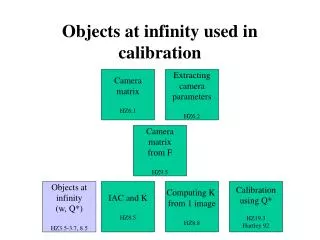
Objects at infinity used in calibration. Camera matrix HZ6.1. Extracting camera parameters HZ6.2. Camera matrix from F HZ9.5. Objects at infinity (w, Q*) HZ3.5-3.7, 8.5. IAC and K HZ8.5. Computing K from 1 image HZ8.8. Calibration using Q* HZ19.3 Hartley 92.

E N D
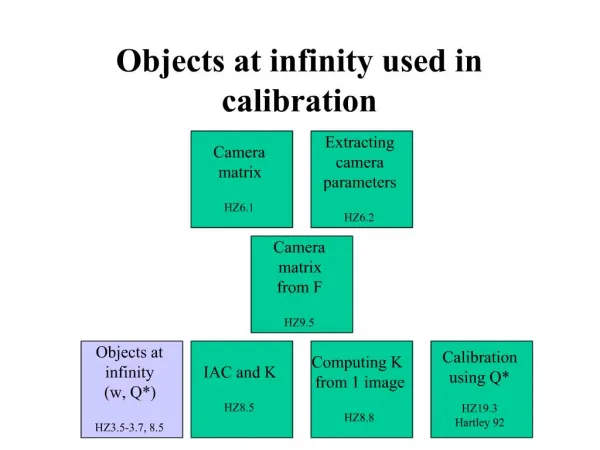
Objects at infinity used in calibration Camera matrix HZ6.1 Extracting camera parameters HZ6.2 Camera matrix from F HZ9.5 Objects at infinity (w, Q*) HZ3.5-3.7, 8.5 IAC and K HZ8.5 Computing K from 1 image HZ8.8 Calibration using Q* HZ19.3 Hartley 92
Thoughts about calibration • now that we have motivated the necessity for moving from projective information about the camera to metric information, we consider calibration of the camera (Chapters 8 and 19) • this requires an understanding of the absolute conic Ω∞(Ch. 3.6-3.7) and the image of the absolute conic or IAC ω (Ch 8.5), as well as the absolute dual quadric Q*∞ • we will start with IAC and develop a method for finding the calibration matrix K using a single image (but also some calibration objects) • later we will show how to develop the entire homography that corrects our camera matrix using IAC and Q*∞ , using two views but no calibration objects • in short: • stage 1: calibration from a single view, using IAC and calibration objects • stage 2: calibration from two views, using IAC and Q*∞ without calibration objects
More thoughts about calibration • the absolute conic Ω∞ -- and its dual, the absolute dual quadric Q*∞ -- are structures that characterize a 3d similarity, like the dual conic did for the 2d similarity • we get interested in images of objects at infinity, since they depend only on camera rotation and calibration matrix K • IAC, a special object at infinity, depends only on K, so it contains the key to solving for K in the calibration stage • IAC and Q*∞ allow angle to be measured in 3-space • given the relationship of IAC and Q*∞ to angle, we can solve for them using angle constraints
Plane at infinity π∞ • once again, we shall be fascinated by objects at infinity • plane at infinity characterizes the affinity • in projective 3-space, points at infinity (x,y,z,0) lie on the plane at infinity π∞ = (0,0,0,1) • two lines (resp., two planes, a line and a plane) are parallel iff intersection lies on π∞ • a projective transformation is an affinity iff π∞ is fixed (as a plane, not pointwise) • i.e., this is a defining invariant of the affinity • identifies the excess: the difference between an affinity (12dof) and a projectivity (15dof) is exactly the 3dof of the plane at infinity π∞ • intuition: once π∞ is known, parallelism is also known, which is a defining invariant of the affinity • can restore parallel lines (think of HW1) • just as angle is a defining invariant of the similarity • i.e., affine rectification involves restoring image of π∞to its rightful position • HZ80-81
The image of π∞ • we are interested in discovering the internal parameters of the camera such as focal length (or computationally in finding K) • to isolate the internal camera parameters, we need to factor out the effects of camera translation and rotation • we get interested in the image of objects at infinity, since these images are independent of the position of the camera • makes sense, since points at infinity are directions, independent of position • the homography between π∞ and the image plane is a planar homography H = KR • proof: consider the image of an ideal point under the camera KR[I –C]: image(d 0) = KR[I –C] (d 0) = KRd • have eliminated the last column’s translation vector • HZ209-210
Absolute conic Ω∞ • absolute conic characterizes the similarity • absolute conic is 3D analogue to circular points (just as π∞ is 3D analogue of L∞ ) • circular points are 0D subset of 1D line at infinity • absolute conic is 1D subset of 2D plane at infinity • conic = plane/quadric intersection • absolute conic Ω∞ = intersection of quadric x2 + y2 + z2 = 0 with plane at infinity • equivalently, absolute conic Ω∞ is represented by the conic with identity matrix I on the plane at infinity • a projective transformation is a similarity iff Ω∞is fixed (as a set) • proof: if A-t I A-1 = kI (so AAt = kI), then mapping A is scaled orthogonal, so represents scaled rotation (perhaps along with reflection) • identifies the excess: difference between a similarity (7dof) and an affinity (12dof) is exactly the 5dof of Ω∞ • HZ81-82
More on absolute conic • metric rectification involves restoring Ω∞ to its rightful position (Charles II) • recall that every circle contains the circular points of its plane • every sphere contains Ω∞ • any circle intersects Ω∞ in 2 points = circular points of the plane that contains the circle • once again, we can measure angle using Ω∞(just as we could with dual of circular points) • and it is invariant to projectivities; but angle measure with next construct Q*∞is better
The image of Ω∞ (aka ω or IAC) • the image of π∞ was good, but the image of Ω∞ (a certain object on the plane at infinity) is even better: it is independent of both position and orientation of the camera • the image of the absolute conic Ω∞ is known by its acronym IAC, and since it is so valued for calibration, it is given its own symbol ω • lowercase ω = uppercase Ω • we’ll call it William • calibration is our end goal and often our last step (so omega) • ω = (KKt)-1 • proof: we saw that the plane at infinity transforms according to the homography KR, so the conic I on the plane at infinity transforms to (KR)-t I (KR)-1 = K-t RR-1 K-1 = (KKt)-1 • since conics map contravariantly (HZ37) and R is orthogonal (Rt = R-1) • conclusion: knowledge of ω implies knowledge of K • HZ210
IAC and circular points • we have seen that circular points lie on the absolute conic, so their image lies on William • this will be used to find William: if we can find enough points on William, we have William • every plane contains 2 circular points • in the plane’s coordinate system, these are (1,i,0) and (1,-i,0) • the plane intersects the plane at infinity in a line at infinity, which intersects the absolute dual conic in 2 points: these are the plane’s circular points • since the plane’s circular points lie on the absolute conic Ω∞, their images lie on the IAC ω • how to find image of circular point? • we shall find the image of a circular point on plane π as H(1,+-i, 0) where H is the homography between π and the image plane • HZ82, 211
Calibrating with calibration objects: 3 squares yield 6 circular points • we shall solve for William (the IAC) by finding 6 circular points that lie on William • you can find points on the vanishing line by intersecting parallel lines • you can find (imaged) circular points by finding a homography (to the image plane) • each planar homography yields 2 points • consider 3 calibration squares in the image on 3 non-parallel planes • assume wlog that the four vertices of each square are (0,0), (1,0), (0,1), (1,1) • aligning the coordinate frame in this way is a similarity • similarity does not affect circular points • HZ211
3-square algorithm • For each calibration square [find 2 points on ω] • Find the corners of the calibration square using user input or automated tracking (see David’s excellent demo). • Use the DLT algorithm to compute the homography H that maps each square vertex to its image [only 4 pts needed]. • Apply this homography to the circular points I and J to find 2 points on ω. • they are h1 +- i h2, where h1 and h2 are first 2 columns of H • Fit ω to 6 points [using numerical computing] • real and imaginary components of x^t ω x = 0 (applied to circular points) yield 2 eqns: • h1tωh2 = 0 • h1tωh1 = h2tωh2 • interesting: the pair of circular points encode the same information, so only one circular point gives useful information; but we still get 2dof because of real and imaginary components (so in effect we are not fitting to 6 points, but getting 6 constraints from 3 pts) • encode these linear equations in Hw = 0 where w is the row-major encoded ω (see development of DLT algorithm) • solve for w (and hence ω) as null vector • Extract calibration matrix K from ω using Cholesky. • ω-1 = KKt • HZ211
Overview of 3-square algorithm • homography of squares to imaged squares 6 imaged circular points (2 per square) image of absolute conic (by fitting) K (by Cholesky factorization) metric properties (see Chapter 19 for how to use K to get metric)