Download
1 / 74
740 likes | 916 Views
Apply KCL to the top node ,we have. We normalize the highest derivative by dividing by C , we get. Since the highest derivative in the equation is 2 , then this equation is. We can not solve this equation by separating variables and integrating as we did in

E N D
We normalize the highest derivative by dividing by C , we get Since the highest derivative in the equation is 2 , then this equation is
We can not solve this equation by separating variables and integrating as we did in The first order equation in Chapter 7 The classical approach is to assume a solution Question : what is a solution we might assume that satisfies the above equation what is a solution that when differentiated twice and added to its first derivative multiplied by a constant and then added to it the solution itself divided by a constant will give zero The only candidate ( مرشح ) that satisfies the above equation will be an exponential functionsimilar to chapter 7
Substituting the proposed or assumed solution into the differential equation we get A ≠ 0 else the whole proposed solution will be zero That leave The equation is called the characteristic equation of the differential equation because the roots of this quadratic equation determine the mathematical character of v(t)
characteristic equation of the differential equation The two roots of characteristic equation are The solutions either one satisfies the differential equation Denoting these two solutions as v1(t) and v2(t)
characteristic equation are solutions regardless of A1 and A2
are solutions Also a combinations of the two solution is also a solution is a solutions as can be shown: Substituting the above in the differential equation , we have is a solutions
are solutions however Is the most general solution because it contain all possible solutions ( Recall how the time constant on RL and RC circuits depend on R,L and C)
characteristic equation of the differential equation Roots of the characteristic equation Rewriting the roots s1,2 as follows: where
characteristic equation of the differential equation where So to distinguish between the two frequencies we name them as
characteristic equation of the differential equation where s1,2 are also frequencies since they are summation of frequencies To distinguish them from the Neper and Resonant frequencies and because s1,2 can be complex we call them complex frequencies All these frequencies have the dimension of angular frequency per timer (rad/s)
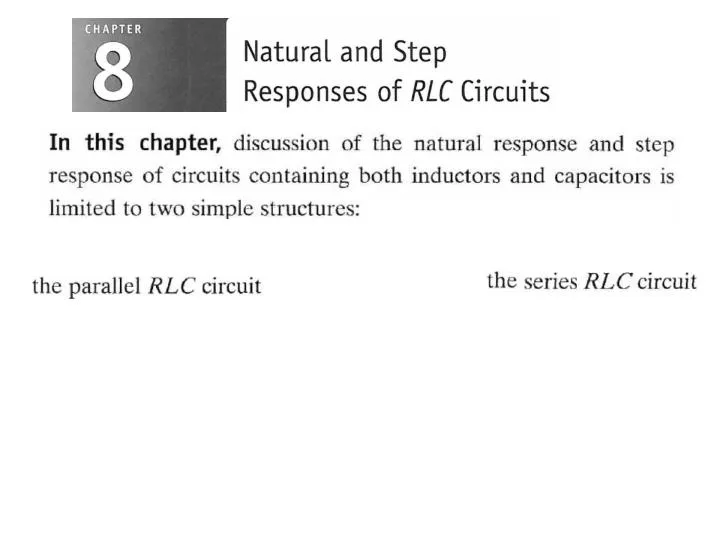
So far we have seen that the behavior of a second-order RLC circuit depends on the values of s1 and s2, which in turn depend on the circuit parameters R,L, and C. Therefore, the first step in finding that natural response is to calculate these values and determine whether the response is overdamped, underdamped or critically damped Completing the description of the natural response requires finding two unknown coefficients, such as A1 and A2 .The method used to do this is based on matching the solution for the natural response to the initial conditions imposed by the circuit In this section, we analyze the natural response form for each of the three types of damping, beginning with the overdamped response as will be shown next
where A1 , A2 are determined from Initial conditions as follows: -------(2) But what is
Summarizing (1) From the circuit elements R,L,C we can find (2)A1 , A2 are determined from Initial conditions as follows: But what is
Because the roots are real and distinct, we know that the response is overdamped
were Damped Radian Frequency Using Euler Identities
It is clear that the natural response for this case is exponentially damped and oscillatory in nature
The constants B1 and B2 are real because v(t) real (the left hand side) Therefore the right hand side is also real The constants A1 and A2 are complex conjugate ( can be shown ) Therefore
Summary were The constants B1 and B2 can be determined from the initial conditions This was shown previously using KCL and Solving (1) and (2) , w obtain B1 and B2
(a) Calculate the roots of the characteristic equation underdamped For the underdamped case, we do not ordinarily solve for s1 and s2because we do not use them explicitly.
The Critically Damped Voltage Response The second-order circuit is critically damped when or where A0 is an arbitrary constant The solution above can not satisfies the two initial conditions (V0, I0) with only on constant A0 It seems that there is a problem ? We can trace this dilemma back to the assumption that the solution takes the form of When the roots of the characteristic equation are equal, the solution for the differential equation takes a different form, namely
The Critically Damped Voltage Response Is not possible assumption because it leads to which can not satisfies (V0, I0 ) Another solution for the differential equation takes a different form, namely The justification of is left for an introductory course in differential equations. Finding the solution involves obtaining D1 and D2 by following the same pattern set in the overdamped and underdamped cases: We use the initial values of the voltage v(0+)and the derivative of the voltage with respect to time dv(0+)/dt to write two equations containing D1 and D2
(a) For the circuit above ,find the value of R that results in a critically damped voltage response. critically damped
(b) Calculate v(t) for t > 0 critically damped
Initial voltage on the Capacitor Initial current through the Indictor
where A1 , A2 are determined from Initial conditions as follows: -------(2)
follows We will show first the indirect approach solution , then the direct approach