Download
1 / 33
330 likes | 364 Views
Exploring MMSE criteria, theorems, and examples for obtaining optimal estimators in terms of observations, focusing on linear and nonlinear approaches.

E N D
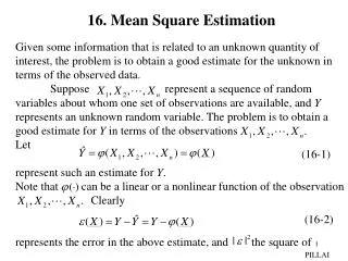
16. Mean Square Estimation Given some information that is related to an unknown quantity of interest, the problem is to obtain a good estimate for the unknown in terms of the observed data. Suppose represent a sequence of random variables about whom one set of observations are available, and Y represents an unknown random variable. The problem is to obtain a good estimate for Y in terms of the observations Let represent such an estimate for Y. Note that can be a linear or a nonlinear function of the observation Clearly represents the error in the above estimate, and the square of (16-1) (16-2) PILLAI
the error. Since is a random variable, represents the mean square error. One strategy to obtain a good estimator would be to minimize the mean square error by varying over all possible forms of and this procedure gives rise to the Minimization of the Mean Square Error (MMSE) criterion for estimation. Thus under MMSE criterion,the estimator is chosen such that the mean square error is at its minimum. Next we show that the conditional mean of Y given Xis the best estimator in the above sense. Theorem1: Under MMSE criterion, the best estimator for the unknown Y in terms of is given by the conditional mean of Y gives X. Thus Proof : Let represent an estimate of Y in terms of Then the error and the mean square error is given by (16-3) (16-4) PILLAI
Since we can rewrite (16-4) as where the inner expectation is with respect to Y, and the outer one is with respect to Thus To obtain the best estimator we need to minimize in (16-6) with respect to In (16-6), since and the variable appears only in the integrand term, minimization of the mean square error in (16-6) with respect to is equivalent to minimization of with respect to (16-5) (16-6) PILLAI
Since X is fixed at some value, is no longer random, and hence minimization of is equivalent to This gives or But since when is a fixed number Using (16-9) (16-7) (16-8) (16-9) PILLAI
in (16-8) we get the desired estimator to be Thus the conditional mean of Y given represents the best estimator for Y that minimizes the mean square error. The minimum value of the mean square error is given by As an example, suppose is the unknown. Then the best MMSE estimator is given by Clearly if then indeed is the best estimator for Y (16-10) (16-11) (16-12) PILLAI
in terms of X. Thus the best estimator can be nonlinear. Next, we will consider a less trivial example. Example : Let where k > 0 is a suitable normalization constant. To determine the best estimate for Y in terms of X, we need Thus Hence the best MMSE estimator is given by y 1 x 1 (16-13) PILLAI
Once again the best estimator is nonlinear. In general the best estimator is difficult to evaluate, and hence next we will examine the special subclass of best linear estimators. Best Linear Estimator In this case the estimator is a linear function of the observations Thus where are unknown quantities to be determined. The mean square error is given by (16-14) (16-15) PILLAI
and under the MMSE criterion should be chosen so that the mean square error is at its minimum possible value. Let represent that minimum possible value. Then To minimize (16-16), we can equate This gives But (16-16) (16-17) (16-18) (16-19) PILLAI
Substituting (16-19) in to (16-18), we get or the best linear estimator must satisfy Notice that in (16-21), represents the estimation error and represents the data. Thus from (16-21), the error is orthogonal to the data for the best linear estimator. This is the orthogonality principle. In other words, in the linear estimator (16-15), the unknown constants must be selected such that the error (16-20) (16-21) PILLAI
is orthogonal to every data for the best linear estimator that minimizes the mean square error. Interestingly a general form of the orthogonality principle holds good in the case of nonlinear estimators also. Nonlinear Orthogonality Rule: Let represent any functional form of the data and the best estimator for Y given With we shall show that implying that This follows since (16-22) PILLAI
Thus in the nonlinear version of the orthogonality rule the error is orthogonal to any functional form of the data. The orthogonality principle in (16-20) can be used to obtain the unknowns in the linear case. For example suppose n = 2, and we need to estimate Y in terms of linearly. Thus From (16-20), the orthogonality rule gives Thus or PILLAI
(16-23) can be solved to obtain in terms of the cross- correlations. The minimum value of the mean square error in (16-17) is given by But using (16-21), the second term in (16-24) is zero, since the error is orthogonal to the data where are chosen to be optimum. Thus the minimum value of the mean square error is given by (16-23) (16-24) PILLAI
where are the optimum values from (16-21). Since the linear estimate in (16-15) is only a special case of the general estimator in (16-1), the best linear estimator that satisfies (16-20) cannot be superior to the best nonlinear estimator Often the best linear estimator will be inferior to the best estimator in (16-3). This raises the following question. Are there situations in which the best estimator in (16-3) also turns out to be linear ? In those situations it is enough to use (16-21) and obtain the best linear estimators, since they also represent the best global estimators. Such is the case if Y and are distributed as jointly Gaussian. We summarize this in the next theorem and prove that result. Theorem2: If and Y are jointly Gaussian zero (16-25) PILLAI
mean random variables, then the best estimate for Y in terms of is always linear. Proof : Let represent the best (possibly nonlinear) estimate of Y, and the best linear estimate of Y. Then from (16-21) is orthogonal to the data Thus Also from (16-28), (16-26) (16-27) (16-28) (16-29) (16-30) PILLAI
Using (16-29)-(16-30), we get From (16-31), we obtain that and are zero mean uncorrelated random variables for But itself represents a Gaussian random variable, since from (16-28) it represents a linear combination of a set of jointly Gaussian random variables. Thus and X are jointly Gaussian and uncorrelated random variables. As a result, and X are independent random variables. Thus from their independence But from (16-30), and hence from (16-32) Substituting (16-28) into (16-33), we get (16-31) (16-32) (16-33) PILLAI
or From (16-26), represents the best possible estimator, and from (16-28), represents the best linear estimator. Thus the best linear estimator is also the best possible overall estimator in the Gaussian case. Next we turn our attention to prediction problems using linear estimators. Linear Prediction Suppose are known and is unknown. Thus and this represents a one-step prediction problem. If the unknown is then it represents a k-step ahead prediction problem. Returning back to the one-step predictor, let represent the best linear predictor. Then (16-34) PILLAI
where the error is orthogonal to the data, i.e., Using (16-36) in (16-37), we get Suppose represents the sample of a wide sense stationary (16-35) (16-36) (16-37) (16-38) PILLAI
stochastic process so that Thus (16-38) becomes Expanding (16-40) for we get the following set of linear equations. Similarly using (16-25), the minimum mean square error is given by (16-39) (16-40) (16-41) PILLAI
The n equations in (16-41) together with (16-42) can be represented as Let (16-42) (16-43) PILLAI
Notice that is Hermitian Toeplitz and positive definite. Using (16-44), the unknowns in (16-43) can be represented as Let (16-44) (16-45) PILLAI
Then from (16-45), Thus (16-46) (16-47) (16-48) PILLAI
and Eq. (16-49) represents the best linear predictor coefficients, and they can be evaluated from the last column of in (16-45). Using these, The best one-step ahead predictor in (16-35) taken the form and from (16-48), the minimum mean square error is given by the (n +1, n +1) entry of From (16-36), since the one-step linear prediction error (16-49) (16-50) (16-51) PILLAI
we can represent (16-51) formally as follows Thus, let them from the above figure, we also have the representation The filter represents an AR(n) filter, and this shows that linear prediction leads to an auto regressive (AR) model. (16-52) (16-53) PILLAI
The polynomial in (16-52)-(16-53) can be simplified using (16-43)-(16-44). To see this, we rewrite as To simplify (16-54), we can make use of the following matrix identity (16-54) (16-55) PILLAI
Taking determinants, we get In particular if we get Using (16-57) in (16-54), with (16-56) (16-57) PILLAI
we get Referring back to (16-43), using Cramer’s rule to solve for we get (16-58) PILLAI
or Thus the polynomial (16-58) reduces to The polynomial in (16-53) can be alternatively represented as in (16-60), and in fact represents a stable (16-59) (16-60) PILLAI
AR filter of order n, whose input error signal is white noise of constant spectral height equal to and output is It can be shown that has all its zeros in provided thus establishing stability. Linear prediction Error From (16-59), the mean square error using n samples is given by Suppose one more sample from the past is available to evaluate ( i.e., are available). Proceeding as above the new coefficients and the mean square error can be determined. From (16-59)-(16-61), (16-61) (16-62) PILLAI
Using another matrix identity it is easy to show that Since we must have or for every n. From (16-63), we have or since Thus the mean square error decreases as more and more samples are used from the past in the linear predictor. In general from (16-64), the mean square errors for the one-step predictor form a monotonic nonincreasing sequence (16-63) (16-64) PILLAI
whose limiting value Clearly, corresponds to the irreducible error in linear prediction using the entire past samples, and it is related to the power spectrum of the underlying process through the relation where represents the power spectrum of For any finite power process, we have and since Thus (16-65) (16-66) (16-67) PILLAI
Moreover, if the power spectrum is strictly positive at every Frequency, i.e., then from (16-66) and hence i.e., For processes that satisfy the strict positivity condition in (16-68) almost everywhere in the interval the final minimum mean square error is strictly positive (see (16-70)). i.e., Such processes are not completely predictable even using their entire set of past samples, or they are inherently stochastic, (16-68) (16-69) (16-70) PILLAI
since the next output contains information that is not contained in the past samples. Such processes are known as regular stochastic processes, and their power spectrum is strictly positive. Power Spectrum of a regular stochastic Process Conversely, if a process has the following power spectrum, such that in then from (16-70), PILLAI
Such processes are completely predictable from their past data samples. In particular is completely predictable from its past samples, since consists of line spectrum. in (16-71) is a shape deterministic stochastic process. (16-71) PILLAI