ENCODING NON LINEAR MIXED EFFECTS MODEL
ENCODING NON LINEAR MIXED EFFECTS MODEL. M arc Lavielle INRIA Saclay. EBI, June 20th, 2011. Population approach & mixed effects model. Some examples of PK/PD data. Daily seizure counts (epilepsy). Viral load CD4 count.


ENCODING NON LINEAR MIXED EFFECTS MODEL
E N D
Presentation Transcript
ENCODING NON LINEAR MIXED EFFECTS MODEL Marc Lavielle INRIA Saclay EBI, June 20th, 2011
Some examples of PK/PD data Daily seizure counts (epilepsy) Viral load CD4 count
Some examples of PK/PD data Daily seizure counts (epilepsy) Viral load CD4 count
Statistical model for continuous data • The model of the observations y is completely defined by : • - The prediction f • The standard deviation g • The distribution of the residual errors e
Statistical model for continuous data The statistical model prediction = f standard deviation = g distribution = normal
Statistical model for continuous data Any application dedicated to a giventaskshouldbe able to understand/interpretthis description of the model The statistical model prediction = f standard deviation = g distribution = normal
Statistical model for continuous data Any application dedicated to a giventaskshouldbe able to understand/interpretthis description of the model The statistical model prediction = f standard deviation = g distribution = normal
Statistical model for continuous data Any application dedicated to a giventaskshouldbe able to understand/interpretthis description of the model The statistical model prediction = f standard deviation = g distribution = normal
Statistical model for continuous data Any application dedicated to a giventaskshouldbe able to understand/interpretthis description of the model The statistical model prediction = f standard deviation = g distribution = normal
Statistical model for time-to-event data The statistical model hazard = l
Statistical model for time-to-event data The statistical model hazard = l
Statistical model for discrete data P(Y=k) , k=1,2,..K Categorical data: Count data: distribution = poisson parameter = lambda Y ~ parametric distribution example: Y ~Poisson(l)
Statistical model of the individual parameters General model:
Statistical model of the individual parameters General model: Linear model:
Statistical model of the individual parameters - Example The statistical model distribution = log-normal standard deviation = omega covariate= c
Statistical model of the individual parameters - Example The statistical model distribution = log-normal standard deviation = omega covariate= c
Defining the statistical model with the MONOLIX GUI • All the information related to the statistical model is stored: • in a Matlab structure • in a XML file • in a « human-readable » script file
<projectname="theophylline_project.xml"> <covariateDefinitionList> <covariateDefinitioncolumnName="WEIGHT" name="t_WEIGHT" transformation="log(cov/70)" type="continuous"/> <covariateDefinitioncolumnName="SEX" type="categorical"> <groupList> <group name="F" reference="true"/> <group name="M"/> </groupList> </covariateDefinition> </covariateDefinitionList> <data columnDelimiter="\t" headers="ID,DOSE,TIME,Y,COV,CAT" uri="%MLXPROJECT%/theophylline_data.txt"/> <models> <statisticalModels> <parameterList> <parametername="ka" transformation="L"> <interceptinitialization="1.000000"/> </parameter> <parametername="V" transformation="L"> <interceptinitialization="1.000000"/> <betaList> <beta covariate="t_WEIGHT" initialization="0"/> </betaList> <variability initialization="1.000000" level="1.000000" levelName="IIV"/> </parameter> <parametername="Cl" transformation="L"> <interceptinitialization="1.000000"/> <variability initialization="1.000000" level="1.000000" levelName="IIV"/> </parameter> </parameterList> <residualErrorModelList> <residualErrorModel alias="const" output="1.000000" outputName="concentration"> <parameterList> <parameter initialization="1.000000" name="a"/> </parameterList> </residualErrorModel> </residualErrorModelList> </statisticalModels>
Coding the (statistical) model with MLXTRAN $DESCRIPTION PK of theophylline $FILE D:/Myproject/theophylline_data.txt $VARIABLES ID, TIME, AMT, OBS use=DV,WT, SEX use=cov type=cat, LW70 = log(WT/70) use=cov $INDIVIDUAL default distribution=log-normal, ka iiv=no, V cov=LW70, Cl, $EQUATION Cc=PKMODEL(ka,V,Cl) $OBSERVATION Concentration type=continuous pred=Cc err=constant