Download
1 / 21
210 likes | 234 Views
Descriptive Statistics: Part One. Farrokh Alemi Ph.D. Kashif Haqqi M.D. Objectives Definitions Sampling methods Types of variables. Reliability and validity Average Median Mode. Table of Content. Objectives.

E N D
Descriptive Statistics: Part One Farrokh Alemi Ph.D. Kashif Haqqi M.D.
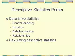
Objectives Definitions Sampling methods Types of variables Reliability and validity Average Median Mode Table of Content
Objectives • Define validity and reliability and explain the role of each in assessing the quality of data. • Distinguish among nominal, ordinal, and numeric data, as well as discrete and continuous data. • Given a set of numerical data, calculate the mean, median and mode, and state the relative advantages of each as a measure of central tendency. Back to Table of Content
Definition of Variables • A variable is an attribute of a person or an object that varies. • Measurement are rules for assigning numbers to objects to represent quantities of attributes. Back to Table of Content
What Is Statistics? • Statistics is the science of describing or making inferences about the world from a sample of data. • Descriptive statistics are numerical estimates that organize and sum up or present the data. • Inferential statistics is the process of inferring from a sample to the population.
Definition • Datum is one observation about the variable being measured. • Data are a collection of observations. • A population consists of all subjects about whom the study is being conducted. • A sample is a sub-group of population being examined.
Sampling Methods • Random sample: all subjects have equal chance of inclusion in the study. • Systematic sampling: selecting the kth numbered subject. • Stratified sample: random sampling within pre-defined groups of subjects. • Staged sampling: A small random sample is made and if its results are ambiguous then another larger random sample is collected. Back to Table of Content
Types of Variables • A discrete variable has gaps between its values. For example, sex is a discrete variable. If male is 1 and female is 0, values in between have no meaning. • A continuous variable has no gaps between its values. All values or fractions of values have meaning. Age is an example of continuous variable. Back to Table of Content
Types of Variables (Continued) • Nominal scale assign numbers to attribute to name the category. The numbers have no meaning by themselves, e.g. DRG code. • Ordinal scale assign numbers so that more of an attribute has higher values, e.g. Severity. • In an interval scale the interval between the numbers has meaning, e.g. Fahrenheit scale • Ratio scale is an interval scale where zero has true meaning, e.g. Age.
Reliability and Validity Back to Table of Content
To Be Valid You Must Have a Reliable Measure. But You Can Have an Invalid Measure That Is Reliable.
Example of Reliability Calculation • Next page shows a table from Hayward, RA, McMahon LF, Bernard AM. Evaluating the care of general medicine inpatients: how good is implicit review? Annals of Internal Medicine, volume 118(7), 1993, pp 550-556. • Two reviewers rated the quality of health care delivered in the same case. The Table shows inter-rater reliability. • 00000605-199304010-00010.
Average • The mean, arithmetic average, is found by adding values of the data and dividing by the number of values. The mean of 3, and 4 is 3.5. • The geometric average is found by multiplying the values of the data and taking the power of one divided by the number of values. The geometric average of 3 and 4 is square root of 3 times 4. • Can you calculate the mean and geometric average for 3, 4, and 5? Back to Table of Content
Example • The mean of 3, 4 and 5 is the sum of these numbers divided by 3. • The geometric average of 3, 4 and 5 is the cube root of 3 times 4 times 5. To calculate the cube root in excel you write a formula like: =(3*4*5)^0.33 • The answer is 3.86. Open Excel and verify that you can do this.
Difference Between Mean and Geometric Average • A geometric average is used when averaging probabilities. • A mean is used in most other context.
Median • The median is the halfway point in a data set. • To calculate median arrange data in order. Calculate half of the observations by dividing the number of values by 2 and rounding the value to the lower number. Count half the values and use the next value as median. Back to Table of Content
Example • The median for age of 7 patients (23, 45, 56, 23, 34, 65, 25) if given by: • Order the list of values: 23, 23, 25, 34, 45, 56, 65. • There are 7 observations. Divide 7 by two and round to lower number and you get 3. • Skip the first 3 and the median is the next number. In this example, 34 is the median. • Do this in Excel.
Mode • The most frequent value observed is the mode. • Mode is always an observed value in the data set. • To calculate the mode, count the number of times each value is repeated. The value with most repetition is the mode. • Do this in Excel. Back to Table of Content
Example for Mode • Age data: 23, 45, 56, 23, 34, 65, 25. • 23 is repeated twice. • All other values are repeated once. • The mode is 23.
Differences in Measures of Central Tendency • Mode, median and mean could be three different numbers in asymmetrical distributions of data. • For any data set there is only one mean and median but there may be many modes. • Median is less influenced by the extreme values than mean. • Mean is almost never observed, median is observed in only odd numbered data sets and mode is always observed in the data set.