Download

1 / 29
290 likes | 339 Views
Learn the principles and procedures of edge detection, including Canny and LOG detectors, characterizing edges, filtering noise, and designing effective edge detectors. Explore Cues of Edge Detection and the Canny Edge Detector theory.

E N D
Course : COMP7116 – Computer Vision Effective Period : February 2018 Edge DetectionSession 06
Learning Objectives • After carefully listening this lecture, students will be able to do the following : • Describe the computational principles underlying various application of Computer Vision Systems • Explain the various standard procedures of image preprocessing prior to image analysis
Outline What is Edge Steps in edge detection Edge detection using derivatives Canny and LOG edge detectors
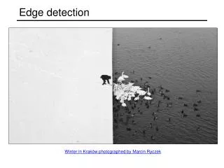
What is edge? Edge is a boundary that is created by the sudden changes (discontinuities) in an image. Edges extract information and used to recognize objects.
Edge Example Edge are caused by a variety of factors
Characterizing Edges An Edge is a place of rapid change in the image intensity function
Effects of noise • Consider a single row or column of the image • Plotting intensity as a function of position gives a signal • Where is the edges?
Effects of noise • Difference filters respond strongly to noise • Image noise results in pixels that look very different from their neighbors • Generally, the larger the noise the stronger the response • What can we do about it?
Solution: Smooth First To find edges, look peaks in
Derivative Theorem of Convolution Differentiation is convolution, and convolution is associative: This saves us one operation:
Tradeoff between Smoothing and Localization Smoothed derivate removes noise, but blurs edge. Also find edges at different “scales”.
Designing an Edge Detector • Criteria for a good edge detector: • Good detection: the optimal detector should find all real edges, ignoring noise or other artifacts • Good localization: • The edges detected must be as close as possible to the true edges • The detector must return one point only for each true edge point • Cues of edge detection • Differences in color, intensity, or texture across the boundary • Continuity and closure • High-level knowledge
Canny Edge Detector J. Canny, A Computational Approach To Edge Detection, IEEE Trans. Pattern Analysis and Machine Intelligence, 8:679-714, 1986. This probably the most widely used edge detector in computer vision Theoretical model: step-edges corrupted by additive Gaussian noise Canny has shown that the first derivative of the Gaussian closely approximates the operator that optimizes the product of signal-to-noise ratio and localization
Get Orientation at Each Pixel • Threshold at minimum level • Get orientation Theta = atan2(gy, gx)
Non-Maximum Suppression for Each Orientation • At q, we have a maximum if the value is larger than those both p and at r. Interpolate to get these values.
Sidebar: Interpolation options • Imx2 = imresize(im, 2, interpolation_type) • “nearest” • Copy value from nearest known • Very fast but creates blocky edges • “bilinear” • Weighted average from four nearest known pixels • Fast and reasonable results • “bicubic” (default) • Non-linear smoothing over larger area (4x4) • Slower, visually appealing, may create negative pixel values
Hysteresis Thresholding Threshold at low/high levels to get weak/strong edge pixels Do connected components, staring from strong edge pixels
Hysteresis Thresholding • Check that maximum value of gradient value is sufficiently large • Drop-outs? Use hysteresis • Use a high threshold to start edge curves and a low threshold to continue them
Canny Edge Detector • Filter image with x, y derivatives of Gaussian • Find magnitude and orientation of gradient • Non-Maximum suppression: • Thin multi-pixel wide “ridges” down to single pixel width • Thresholding and linking (hysteresis): • Define two thresholds: low and high • Use the high threshold to start edge curves and he low threshold to continue them • MATLAB: edge(image, ‘canny’)
Exercise Jalankan demo deteksibantengdengan edge detection,ekstrasksi contour, image feature dan histogram equalization
References Richard Szeliski. (2011). Computer Vision: Algorithms and applications. 01. Springer. Chapter 4. David Forsyth and Jean Ponce. (2002). Computer Vision: A Modern Approach. 02. Prentice Hall. Chapter 8. https://cs.brown.edu/courses/cs143/lectures/07.pdf